Algorithmic number theory
Relevant readings: CLRS 31.8–31.9, Katz and Lindell 9.2, 10.1–10.2, App. B
Primality testing
Distribution of primes
Recall from Lecture 3 that although there’s no clear pattern about the distribution of prime numbers, one of the great insights about them is that their density among the integers has a precise limit, which is described by the prime number theorem.
The approximation \(n / \ln n\) gives reasonably accurate estimates of \(\pi(n)\) even for small \(n\). For example, it is off by less than \(6%\) at \(n = 10^9\), where \(\pi(n) = 50847534\) and \(n/ \ln n = 48 254942\).
By the prime number theorem, the probability that \(n\) is prime is approximately \(1 / \ln n\), and so we would expect to examine approximately \(\ln n\) integers chosen randomly near \(n\) in order to find a prime that is of the same length as \(n\). For example, we expect that finding a \(1024\)-bit prime would require testing approximately \(\ln 2^{1024} \approx 710\) randomly chosen \(1024\)-bit numbers for primality. Of course, we can cut this figure in half by choosing only odd integers.
Fermat’s pseudoprime test
We now consider a method for primality testing that “almost works” and in fact is good enough for many practical applications.
Recall that Fermat’s little theorem says that for any integer \(a>0\) and prime \(n\), $$a^{n-1} \equiv 1 \pmod{n}. \label{eq:fermat_little}$$
However, if \(n\) is composite and still satisfies the above equation, then we say that \(n\) is a base-\(a\) pseudoprime. Thus, if we can find any \(a\) such that \(n\) does not satisfy the equation, then \(n\) is certainly composite. Surprisingly, the converse almost holds, so that this criterion forms an almost perfect test for primality. We test to see whether \(n\) satisfies equation [eq:fermat_little] for \(a = 2\). If not, we declare \(n\) to be composite by returning “composite.” Otherwise, we return “prime,” guessing that \(n\) is prime, when in fact, all we know is that \(n\) is either prime or a base-\(2\) pseudoprime.
FermatTest(\(n\)):
1: if FastModExp\((a, n-1, n) \ne 1\) // if \(a^{n-1} \not\equiv 1 \pmod{n}\)
2: return “composite” // definitely
3: else
4: return “prime“ // perhaps
This algorithm can make errors, but only of one type. That is, if it says that \(n\) is composite, then it is always correct. If it says that \(n\) is prime, however, then it makes an error only if \(n\) is a base-\(2\) pseudoprime.
How often does this algorithm output the wrong answer? Surprisingly rarely. There are only \(22\) values of \(n\) less than \(10000\) for which it is wrong; the first four such values are \(341\), \(561\), \(645\), and \(1105\). We won’t prove it, but the probability that this algorithm makes an error on a randomly chosen \(m\)-bit number goes to zero as \(m \to \infty\).
The upshot is that if you are merely trying to find a large prime for some application, for all practical purposes you almost never go wrong by choosing large numbers at random until one of them causes FermatTest to return “prime.” But when the numbers being tested for primality are not randomly chosen, we need a better approach for testing primality.
Miller–Rabin primality test
The Miller–Rabin primality test overcomes the problems of the simple Fermat’s pseudoprime test with two modifications:
-
It tries several randomly chosen base values \(a\) instead of just one base value.
-
While computing each modular exponentiation, it looks for a nontrivial square root of \(1\) modulo \(n\), during the final set of squarings. If it finds one, it stops and returns “composite.”
MillerRabin(\(n\), \(t\)):
1: for \(j \gets 1 \ \textbf{to}\ t\)
2: \(a \getsrandom \Set{1, \dots, n-1}\)
3: if Witness(\(a\), \(n\))
4: return “composite” // definitely
5: return “prime” // almost surely
Integer factorization
Suppose we have an integer \(n\) that we wish to factor, that is, to decompose into a product of primes. The primality test of the preceding section may tell us that \(n\) is composite, but it does not tell us the prime factors of \(n\). Factoring a large integer \(n\) seems to be much more difficult than simply determining whether \(n\) is prime or composite. Even with today’s supercomputers and the best algorithms to date, we cannot feasibly factor an arbitrary \(1024\)-bit number.
Trial division
The most straightforward way to factor an integer \(n\) is to try every possible factor; this is called trial division. We try dividing \(n\) by each integer \(2, 3, \dots, \lfloor \sqrt{n} \rfloor\). (We may skip even integers greater than 2.) It is easy to see that \(n\) is prime if and only if none of the trial divisors divides \(n\). Assuming that each trial division takes constant time, the worst-case running time is \(O(\sqrt{n})\), which is exponential in the length of \(n\).
Pollard’s \(\rho\) algorithm
Pollard’s \(\rho\) (“rho”) algorithm can be used to factor an arbitrary integer \(n = pq\); in that sense, it is a general-purpose factoring algorithm. The core idea of the approach is to find distinct values \(x, x^\prime \in \ZZ_n^*\) that are equivalent modulo \(p\) (that is, if \(x \equiv x^\prime \pmod{p}\)); we call such a pair good. Note that for a good pair \(x, x^\prime\) it holds that \(\gcd(x-x^\prime, n ) = p\), since \(x \not\equiv x^\prime \pmod{n}\), so computing the gcd gives a nontrivial factor of \(n\).
The algorithm involves generating a pseudorandom sequence, which is done by a function \(f\). In other words, we will keep applying \(f\) and it will generate numbers that “look and feel” random. (Note that it can never be truly random because this entire sequence can be determined from the choice of \(f\) and the starting value.) Not every function does it but one such function that has this pseudorandom property is \(f(x) \gets (x^2+c) \bmod n\), where \(c\) is usually assumed to be \(1\) in practice.
We define our starting value to be \(x_0 \gets 2\), but any other integer could work. To get the next element \(x_1\) in the sequence, we compute \(x_1 \gets f(x_0)\), and to get the element after that \(x_2\), we compute \(x_2 \gets f(x_1)\). In general, we have the recurrence \(x_{i+1} \gets f(x_i)\).
Suppose \(n = 95\) and \(f(x) \gets (x^2+1) \bmod n\). We show how to derive the pseudorandom sequence in the following table:
| \(x_i\) | \(x_{i+1}\) | \(g \gets \gcd(\abs{x_i - x_{i-1}}, n)\) |
|---|---|---|
| \(2\) | \(5\) | \(\gcd(3, 95) = 1\) |
| \(5\) | \(26\) | \(\gcd(21, 95) = 1\) |
| \(26\) | \(12\) | \(\gcd(14, 95) = 1\) |
| \(12\) | \(50\) | \(\gcd(38, 95) = 19\) |
The last pair of \(x_i, x_{i+1}\) is good since the last value of \(g\) is greater than \(1\), so this must be a nontrivial factor of \(n\). Thus we have found \(19\) as a prime factor of \(95\).
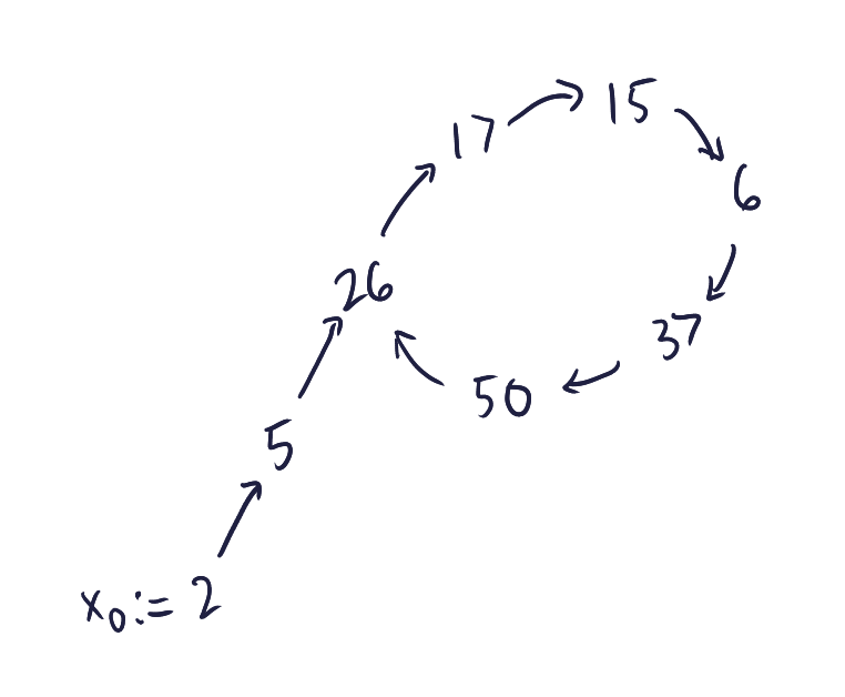
You can see that in many cases this works. But in some cases, it goes into an infinite loop because the function \(f\) gets trapped into a cycle. When that happens, we keep repeating the same set of value pairs \(x_i\) and \(x_{i+1}\) and never stop. For example, if \(n = 55\) and \(f\) is the same as defined previously, the pseudorandom sequence would be: $$2, 5, \textcolor{tomred}{26, 17, 15, 6, 37, 50, 26}, 17, 15, 6, 37, 50, 26, 17, 15, 6, \dots.$$ In this case, we will keep cycling and never find a factor. How do we detect that there is a cycle?
A simple solution is to store all the numbers seen so far \(x_1, \dots, x_n\) in some data structure, and see if \(x_i = x_j\) for some previous \(i < j\). However, doing so would take \(O(n)\) memory, and for very large values of \(n\) (as it usually is in practice) it is infeasible.
A more efficient solution relies on another algorithm to find cycles called Floyd’s algorithm. We have already seen how Floyd’s algorithm works in the context of finding hash collisions, but the idea remains the same:
PollardRho(\(n\)):
1: \(\textit{tortoise} \gets x_0\)
2: \(\textit{hare} \gets x_0\)
3: \(\textit{tortoise} \gets f(\textit{tortoise})\) // tortoise moves one step forward
4: \(\textit{hare} \gets f(f(\textit{hare}))\) // hare moves two steps forward
5: \(g \gets \gcd(\abs{\textit{tortoise} - \textit{hare}}, n)\)
6: if \(1 < g < n\)
7: return \(g\)
8: else if \(g \mathrel{=}n\)
9: return “fail”
The running time of Pollard’s \(\rho\) algorithm turns out to be \(O(\sqrt{p})\) where \(p\) is the smallest divisor that divides \(n\). If \(p\) just so happens to be really small, this algorithm is practically efficient no matter how enormous \(n\) can be. But in the worst case, \(n\) is a product of two equally-sized prime factors, so each of the factors has half the number of bits of \(n\), which means that the running time in terms of \(n\) will be \(O(n^{1/4})\).
Fun fact: The main reason why this algorithm is called the \(\rho\) algorithm is because of the shape that the pseudorandom sequence produces:
Computing discrete logarithms
Let \(G\) be a cyclic group of known order \(q\). An instance of the discrete logarithm problem in \(G\) specifies a generator \(g \in G\) and an element \(h \in G\); the goal is to find \(x \in \ZZ_q\) such that \(g^x = h\).
A trivial brute-force solution can be done in \(O(q)\) time by iterating through every possible value of \(x\):
NaïveDLog(\(g\), \(h\), \(q\)):
1: for \(x \gets 0 \ \textbf{to}\ q-1\)
2: if \(g^x \mathrel{=}h\)
3: return \(x\)
4: return “fail”
Note that this runs in time exponential to the number of bits of \(q\).
Baby-step giant-step algorithm
A more efficient way to compute discrete logarithms is called the baby-step giant-step algorithm, attributed to Daniel Shanks, which is actually a slight modification of the straightforward solution above. This algorithm is based on a time–memory trade-off, which reduces computing time but comes at the expense of additional memory consumption.
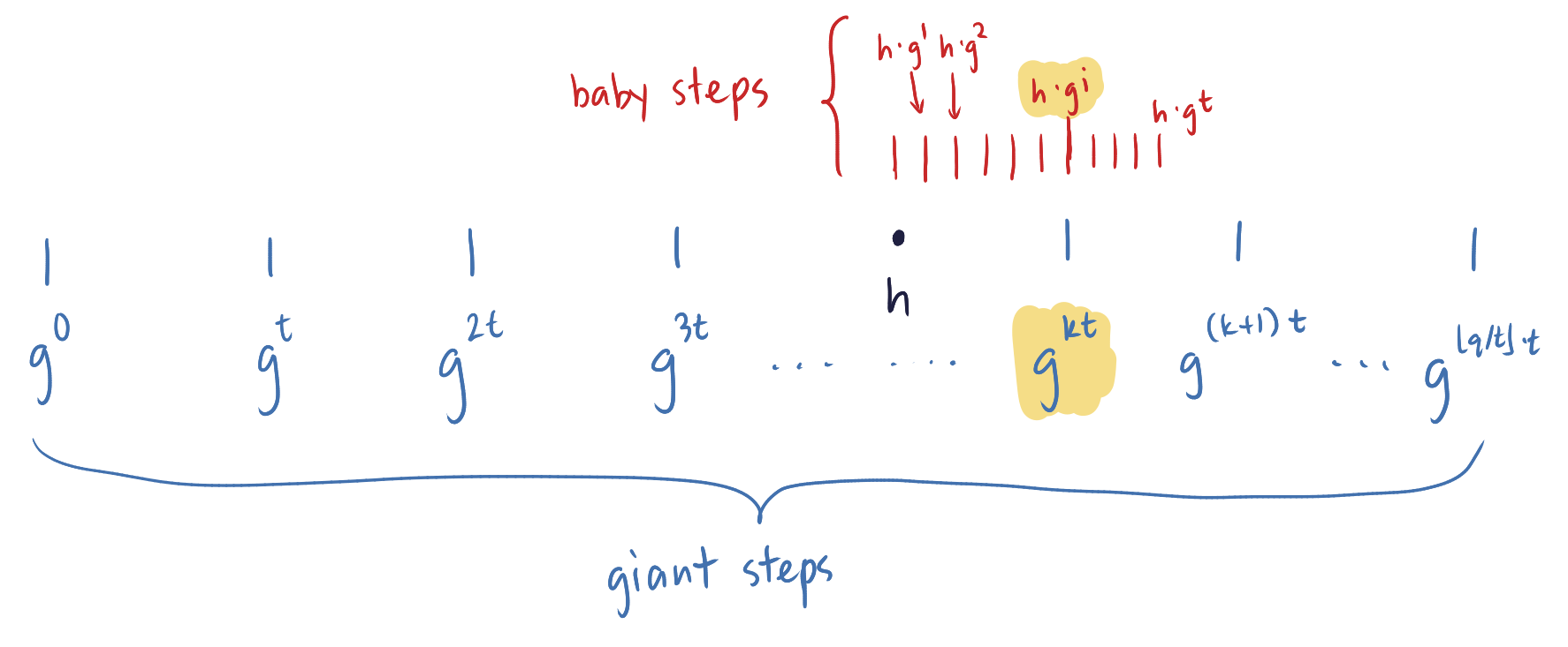
The idea is simple. Given a generator \(g \in G\), we can imagine the powers of \(g\) as forming a cycle $$1 = g^0, g^1, g^2, \dots, g^{q-2}, g^{q-1}, g^q = 1.$$ We know that \(h\) must lie somewhere in this cycle. Computing all the points in this cycle to find \(h\) would take at least time linear in \(q\). Instead, we “mark off” the cycle at intervals of size \(t \gets \lfloor \sqrt{q} \rfloor\). More precisely, we compute and store the \(\lfloor q/t \rfloor + 1 = O(\sqrt{q})\) elements $$g^0, g^t, g^{2t}, \dots, g^{\lfloor q/t \rfloor \cdot t}.$$ These elements are the “giant steps.” Note that the gap between any consecutive “marks” (wrapping around at the end) is at most \(t\). Furthermore, we know that \(h = g^x\) lies in one of these gaps. Thus, if we take “baby steps” and compute the \(t\) elements $$h \cdot g^1, h \cdot g^2, \dots, h \cdot g^t,$$ each of which corresponds to a “shift” of \(h\), we know that one of these values will be equal to one of the marked points. Suppose we find \(h \cdot g^i = g^{k \cdot t}\). We can then easily compute \(\log_g h \gets (k\cdot t - i) \bmod q\).
The following pseudocode summarizes this strategy:
BSGS(\(g\), \(h\), \(q\)):
1: \(t \gets \lfloor \sqrt{q} \rfloor\)
2: for \(i \gets 0 \ \textbf{to}\ \lfloor q/t \rfloor\) // giant step
3: \(g_i \gets g^{i \cdot t}\)
4: store the pair \((i, g_i)\) in a lookup table
5: sort the lookup table by the second component // sort by \(g_i\)
6: for \(i \gets 1 \ \textbf{to}\ t\) // baby step
7: \(h_i \gets h \cdot g^i\)
8: if \(h_i \mathrel{=}g_k\) for some \(k\) // use the lookup table to do this
9: return \((k \cdot t - i) \bmod q\)
10: return “fail” // discrete log does not exist
Since \(t = O(\sqrt{q})\), the algorithm runs in \(O(\sqrt{q})\) time, but it also consumes \(O(\sqrt{q})\) space due to the lookup table. Though this seems like a massive improvement over the naïve discrete log algorithm, keep in mind that this still runs in exponential time in the number of bits of \(q\).
References
-
Cormen, Thomas H., Charles E. Leiserson, Ronald L. Rivest, and Clifford Stein. 2009. Introduction to Algorithms. 3rd ed. MIT Press.
-
Katz, Jonathan, and Yehuda Lindell. 2021. Introduction to Modern Cryptography. 3rd ed. CRC Press.