Stream ciphers
Relevant readings: Aumasson ch. 5
Introducing stream ciphers
Stream ciphers take two values: a key and a nonce (which stands for “number used only once”),1 and produce a pseudorandom stream of bits called the keystream. The key should be secret and is usually \(128\) or \(256\) bits. The nonce doesn’t have to be secret, but it should be unique for each key and is usually between \(64\) and \(128\) bits.
Encryption and decryption work similarly to the one-time pad: the keystream is XOR’ed with the plaintext to encrypt it, and the ciphertext is XOR’ed with the keystream to decrypt it. More concretely, a stream cipher produces a keystream \(\textit{KS} = \textsf{SC}(K, N)\) given a secret key \(K\) and a public nonce \(N\), encrypts as \(C = P \oplus \textit{KS}\), and decrypts as \(P = C \oplus \textit{KS}\).
Stateful and counter-based stream ciphers
Stream ciphers generally belong into two main types: stateful and counter-based.
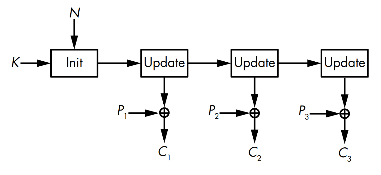
From the name itself, a stateful stream cipher uses an internal state to facilitate the generation of the keystream. It sets up the initial state using the key and the nonce, and then uses the update function to update the state and produce a keystream bit, as shown in Figure 1.
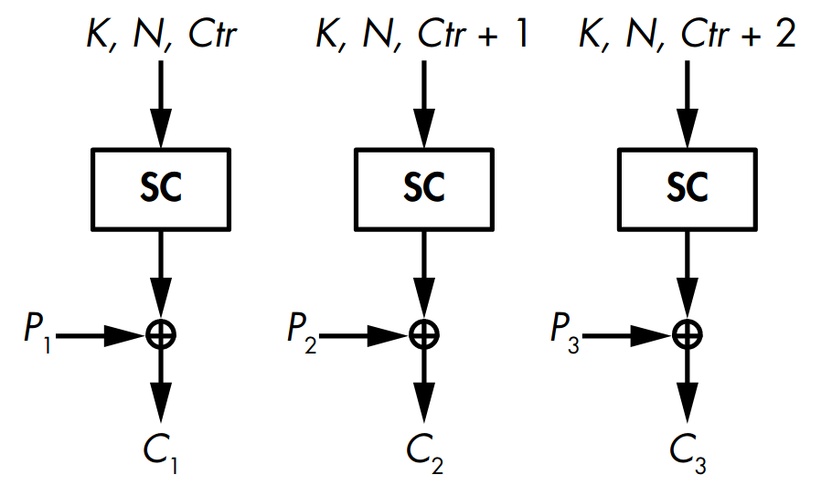
A counter-based stream cipher produces chunks of keystream from a key, a nonce, and a counter value, as shown in Figure 2.
Hardware and software implementations
A cipher’s hardware implementation refers to the dedicated electronic circuit that implements the cryptographic algorithm. These usually come in the form of application-specific integrated circuits (ASICs), programmable logic devices (PLDs), and field-programmable gate arrays (FPGAs). As such, these can’t be used for anything else other than the cryptographic algorithm itself. On the other hand, a software implementation is just a set of instructions to be executed by a microprocessor.
A notable difference between hardware and software implementations is that hardware-based ciphers deal with bits, while software-based ciphers deal with bytes or words (\(32\) or \(64\) bits depending on the processor).
Feedback shift registers
Feedback shift registers (FSRs) are the simplest hardware stream ciphers. Under the hood they are just an array of bits equipped with a feedback function.
Let \(R_0\) be the initial value of the FSR. Then the next state \(R_1\) is defined as \(R_0\) left-shifted by \(1\) bit. The bit that got pushed out the register is returned as output, while the newly emptied position is filled with \(f(R_0)\).
This process is then repeated for the next state values. Given the current state of the FSR \(R_t\), the next state \(R_{t+1}\) can be computed using the following recurrence: $$R_{t+1} = (R_t \shl 1) \BitOr f(R_t)$$ where \(\BitOr\) is the bitwise OR operator and \(\shl\) is the left shift operator.
Suppose we have a \(4\)-bit FSR, whose feedback function \(f\) takes
the XOR of all four bits, and the state is initialized as 1100. To get
the next state, we shift the bits to the left and then set the rightmost
bit as
\(f(\texttt{1000}) = \texttt{1} \oplus \texttt{0} \oplus \texttt{0} \oplus \texttt{0} = \texttt{1}\).
Thus the state becomes 0001 and it outputs 1.
We repeat this process three more times to produce three more keystream
bits, which gives the state values 0011, 0110, and 1100.
Notice that we return to our initial state 1100 after five iterations,
so we say that \(5\) is the period of the FSR. Naturally we would
want a longer period and less repeating patterns for better security.
Linear feedback shift registers
Linear feedback shift registers (FSRs) are FSRs with a linear feedback function. Usually such functions involve XOR’ing some bits of the state, just like the feedback function presented in the previous example. We refer to the bits that influence the input as taps.
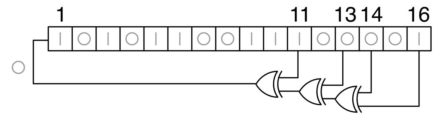
LFSRs use the arithmetic over the finite field \(\FF_{2^n}\), represented as polynomials whose coefficients are either \(0\) or \(1\). The feedback function then is a polynomial expression that encodes which bits are used as taps, specifically for an \(n\)-bit LFSR uses the feedback polynomial $$\sum_{i=0}^n x^i = x^n + \cdots + x^2 + x + 1$$ where the term \(x^i\) is only included if the \(i\)th bit is a tap. For example, the LFSR shown in Figure 3 uses bits \(11\), \(13\), \(14\), and \(16\) as taps, so its feedback polynomial is $$x^{16} + x^{14} + x^{13} + x^{11} + 1.$$ The “\(1\)” in the polynomial doesn’t actually correspond to a tap, but rather, it corresponds to the input to the first bit. As a rule of thumb, the feedback polynomial of an \(n\)-bit LFSR always contains a “\(1\)” and an “\(x^n\)” term.
Every polynomial \(f(x)\) with coefficients in \(\FF_2\) having \(f(0) = 1\) divides \(x^m + 1\) for some \(m\). The smallest \(m\) for which this is true is called the period of \(f(x)\). It’s also helpful to know that an irreducible polynomial of degree \(n\) has a period which divides \(2^n - 1\), and an irreducible polynomial of degree \(n\) whose period is \(2^n - 1\) is called a primitive polynomial.2 To find a suitable feedback polynomial for an \(n\)-bit LFSR, we can use the following theorem (which we won’t prove here):
An \(n\)-bit LFSR is maximal iff its feedback polynomial is a primitive polynomial of degree \(n\) over \(\FF_{2}\).
-
\(x^4 + x^3 + x^2 + 1\) is not irreducible over \(\FF_2\) since we can factor it as \((x+1)(x^3+x+1)\).
-
\(x^4 + x^3 + x^2 + x + 1\) is irreducible over \(\FF_2\) since it has no linear factors. But \(x^5 + 1 = (x+1) (x^4 + x^3 + x^2 + x + 1)\) so it has period \(5\), and \(5 \ne 2^4 - 1 = 15\) so it is not a primitive polynomial.
-
\(x^4 + x^3 + 1\) is irreducible over \(\FF_2\). Thus it has a period which divides \(2^4-1 = 15\); its divisors are \(1, 3, 5, 15\). Since the period must be greater than \(4\), there are two possible values: \(5\) and \(15\). We try each value and get the following: $$\begin{align} x^5 + 1 &= (x+1) (x^4 + x^3 + 1) + (x^3+x) \\ x^{15} + 1 &= (x^{11} + x^{10} + x^9 + x^8 + x^6 + x^4 + x^3 + 1) (x^4 + x^3 + 1) \end{align}$$
Therefore \(x^4 + x^3 + 1\) has period \(15\), so it is a primitive polynomial.
If we want to achieve the maximal LFSR, these conditions are then necessary (but not sufficient):
-
There must be an even number of taps.
-
The set of taps are relatively prime to each other, meaning if we have the set of taps \(\Set{t_1, \ldots, t_m}\) then \(\gcd(t_1, \ldots, t_m) = 1\).
SageMath has bulit-in functionality for constructing LFSRs:
FF = GF(2)
P.<x> = PolynomialRing(FF)
lfsr = LFSRCryptosystem(FF)
# cast each element in the list as elements of GF(2)
init_state = list(map(FF, [0,1,1,0,1,1,0,1,0,1]))
fb = x^10 + x^8 + x^5 + x^4 + 1
# if fb is primitive then our LFSR is maximal
fb.is_primitive()    # ==> True
e = lfsr((fb, init_state))
# generate 32 bytes worth of zeros
m = e.domain().encoding('\x00'*32)
# output first 32 bytes of the keystream
e(m)
Using an LFSR as a stream cipher on its own is insecure, as an attacker only needs \(2n\) output bits to recover the initial state of an \(n\)-bit LFSR and allow them to determine the previous and future bits. This is carried out using the Berlekamp–Massey algorithm that solves the equations defined by the LFSR’s mathematical structure to recovers the initial state and the feedback polynomial. You can even do this attack using SageMath:
# yoinked somewhere in the middle
ks = [0,0,0,0,1,1,1,1,0,0,0,0,0,1,1,0,0,1,1,1]
from sage.matrix.berlekamp_massey import berlekamp_massey
berlekamp_massey(list(map(GF(2), ks)))
It is important to note that LFSRs are not cryptographically secure because they are linear, and so output bits and initial state bits can be recovered using techniques from linear algebra.3 To work around this problem, stuff such as nonlinearity is introduced to strengthen LFSRs.
A5/1
A5/1 is a stream cipher that was used to encrypt voice communications in the GSM mobile standard.
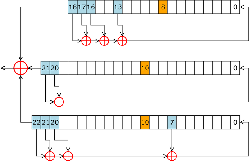
It uses three LFSRs with \(19\), \(22\), and \(23\) bits (as shown in Figure 4) where the feedback polynomials for each as follows: $$\begin{align} &x^{19} + x^{18} + x^{17} + x^{14} + 1 \\ &x^{22} + x^{21} + 1 \\ &x^{23} + x^{22} + x^{21} + x^8 + 1\end{align}$$
Unlike the typical LFSRs, its update mechanism is different. Instead of updating all three LFSRs at each clock cycle, the designers of A5/1 added a clocking rule that does the following:
-
Check the value of the ninth bit of LFSR 1, the \(11\)th bit of LFSR 2, and the \(11\)th bit of LFSR 3, called the clocking bits. Of those three bits, either all have the same value (
1or0) or exactly two have the same value. -
Clock the registers whose clocking bits are equal to the majority value,
0or1. Either two or three LFSRs are clocked at each update.
A5/1 is vulnerable to known-plaintext attacks since these attacks also recover the 64-bit initial state of the system (i.e., all of the initial states of the three LFSRs), which reveals the \(22\)-bit nonce and the \(64\)-bit key used by GSM.
By 2010, it became possible to decrypt calls encrypted with A5/1 in near-real time, so telcos tried to mitigate such attacks, and thus a push to come up with a real solution. Later standards such as 3G and LTE ditched A5/1 altogether.
RC4
RC4 is a stream cipher designed by Ron Rivest in 1987. Unlike LFSRs, RC4 is more suited to be implemented in software as it does not use any other operations than addition and swapping. Originally a trade secret, the source code of RC4 was anonymously posted in 1994, and then was leaked and reverse-engineered within days.4 RC4 was notably used in the very first Wi-Fi encryption protocol called Wired Equivalent Privacy (WEP)5 and in the Transport Layer Security (TLS) protocol. We will see later why RC4 is no longer secure enough for most applications today.
How RC4 works
RC4 maintains an internal state, which consists of an array \(S\) representing one of the possible permutations of all \(256\) bytes, initially set to \(S[0] = 0\), \(S[1] = 1\), …, \(S[255] = 255\). Using a key scheduling algorithm, \(S\) is then initialized based on the supplied key \(K\).
KSA(\(K\)):
1: for \(i :=0 \ \textbf{to}\ 255\)
2: \(S[i] :=i\)
3: \(j :=0\)
4: for \(i :=0 \ \textbf{to}\ 255\)
5: \(j :=(j + S[i] + K[i \bmod K.\textit{length}]) \bmod 256\)
6: swap \(S[i]\) with \(S[j]\)
The keystream, which is of the same length as the plaintext, is then generated using a pseudorandom generator.
PRG(\(m\)):
1: \(i :=0\)
2: \(j :=0\)
3: for \(b :=0 \ \textbf{to}\ m-1\)
4: \(i :=(i+1) \bmod 256\)
5: \(j :=(j+ S[i]) \bmod 256\)
6: swap \(S[i]\) with \(S[j]\)
7: \(\textit{KS}[b] :=S[(S[i] + S[j]) \bmod 256]\)
Suppose we have an all-zero \(128\)-bit as the key. Running the key scheduling algorithm, \(S\) would now become $$[0, 35, 3, 43, 9, 11, 65, 229, \ldots, 233, 169, 117, 184, 31, 39]$$ If we want to generate a \(10\)-byte keystream, running the pseudorandom generator yields: $$[222, 24, 137, 65, 163, 55, 93, 58, 138, 6].$$
Although many people back then considered RC4 “too simple to be broken,” it didn’t stop them from finding exploitable weaknesses.
RC4 as used in WEP
WEP was the very first security protocol for Wi-Fi since the IEEE 802.11 standard was first released in 1997, and for some time this was the only form of security available for Wi-Fi routers supporting the 802.11a and 802.11b standards.
Within the implementation of WEP, RC4 was used as its pseudorandom generator. Unlike most stream ciphers, RC4 did not take a nonce as input, so the workaround was to concatenate it with the secret key, and then feed that to RC4 as the seed. That is, the key \(K\) is appended to the \(24\)-bit nonce \(N\), the actual RC4 key used is \(N \mathrel{\hspace{1pt}||\hspace{1pt}}K\). As a result, the \(128\)-bit WEP protocol actually offers only \(104\)-bit security, and the weaker \(64\)-bit WEP actually offers only \(40\)-bit security!
But that’s not the only problem about WEP:
-
Since the nonce is only \(24\) bits long, there are \(2^{24} = 16777216\) possible choices. This means it only took a few megabytes’ worth of traffic until two packets are encrypted with the same nonce. The attacker can intercept these two packets and do a known-plaintext attack to recover the other message.
-
Combining the nonce and key in this fashion helps recover the key. Since the nonce is publicly-viewable, it is possible to determine the value of \(S\) after three iterations of the key scheduling algorithm.
These weaknesses allow for known-plaintext and chosen-plaintext attacks
against WEP. Not only these attacks are possible in theory, these are
very much possible in practice (e.g., tools like aircrack-ng implement
the entire attack). Further refinements have lessened the number of
captured packets needed to carry out the attack.6
Thus WEP was eventually deprecated in 2004, by which Wi-Fi Protected Access (WPA) and WPA2 were made available as replacements with the ratification of the full 802.11i standard.
Segue: Why did old schemes use keys that are too short?
Believe it or not, the main reason was not because of the limitations of technology at that time.
Here’s a quick history of cryptography policy, at least in the United States. In the Cold War era, cryptography was almost exclusively used by the military, so encryption technology (which eventually included cryptography software) was included into the United States Munitions List in 1954, which put basically everything that uses cryptography in the same league as missiles, bombs, grenades, and flamethrowers. This means the export of cryptography outside the US was severely restricted and heavily regulated for reasons involving national security.7
As cryptography became increasingly widespread in non-military applications, namely for commercial usage, these restrictions became problematic. For example, Netscape released two versions of its browser: one for the US market that supported “full-size” keys (such as \(128\)-bit RC4), and another one for the rest of the world that used reduced key lengths (such as \(40\)-bit RC4). This was also the case for WEP, where two versions are released, namely WEP-40 and WEP-104.
It wasn’t until the late 1990s when these export restrictions were gradually eased, due to legal challenges brought by privacy advocates, though some restrictions still remain today.8
Stream ciphers gone wrong
Nonce reuse
The most common mistake involving stream ciphers is when a nonce is reused with the same key. This is similar to when you reuse the key in a one-time pad: once you have two ciphertexts, you can XOR them together to get the XOR of the two plaintexts, where the identical keystreams cancel each other out in the process.
Broken RC4 implementation
Here’s yet another reason why you don’t implement cryptographic algorithms from scratch. If you were to implement RC4 on your own, there’s a chance that you an already weak cipher even weaker!
Typically, you would implement a swap operation involving \(S[i]\) and \(S[j]\) by using a temporary variable like this:
1: \(\textit{temp} :=S[i]\)
2: \(S[i] :=S[j]\)
3: \(S[j] :=\textit{temp}\)
This is fine, but if space is at a premium you would want to avoid using additional variables as much as possible. Another way that some programmers do is to use a piece of black magic called an XOR swap:
1: \(x :=x \oplus y\)
2: \(y :=x \oplus y\)
3: \(x :=x \oplus y\)
This works since the second line sets \(y\) to \((x \oplus y) \oplus y = x\) and the third line sets \(x\) to \((x \oplus y) \oplus (x \oplus y \oplus y) = y\).
Now take a moment to see what could go wrong if we do the XOR swap for \(S[i]\) and \(S[j]\) (try it by plugging your own values of \(i\) and \(j\)):
1: \(S[i] :=S[i] \oplus S[j]\)
2: \(S[j] :=S[i] \oplus S[j]\)
3: \(S[i] :=S[i] \oplus S[j]\)
What if \(i\) is equal to \(j\)? Instead of leaving the state unchanged, the XOR swap will set \(S[i]\) to \(S[i] \oplus S[i] = 0\), so a byte of the state will be set to zero each time \(i\) equals \(j\) in the key scheduling algorithm and in the pseudorandom generator. Repeat this enough and this would eventually lead to all-zero state and thus to an all-zero keystream. Yikes!
The moral of the story here is to not fix what’s not broken (i.e., do not over-optimize your implementation) and that sometimes the best solution is the simplest one.
References
- Aumasson, Jean-Philippe. 2017. Serious Cryptography: A Practical Introduction to Modern Encryption. No Starch Press.
In the context of stream ciphers, a nonce is also called an initialization vector (IV).
This is pretty similar to the notion of generators in group theory.
For example, Gauss–Jordan elimination works in any field, whether \(\RR\) or \(\FF_2\).
Naturally, this led to a “chilling effect” that prevented academic cryptographers from publishing their research, because doing so would violate these export laws.