Notes for CSCI 184.03
Lecture notes by Brian Guadalupe
This is the online version of the PDF lecture notes I created for this course. These have been converted from the original LaTeX source files to Markdown using Pandoc, and transformed into an online book using mdbook. Some parts have been modified to add interactivity, e.g., using SageMathCell for Sage code.
These online notes still have rough edges. If you see any typos or issues, please let me know!
Contents
-
Introduction
-
Math Background
-
Symmetric-Key Cryptography
-
Public-Key Cryptography
References
These notes are, for the most part, based on these references:
- Jean-Philippe Aumasson. Serious Cryptography: A Practical Introduction to Modern Encryption. No Starch Press, 2017.
- Jonathan Katz and Yehuda Lindell. Introduction to Modern Cryptography. CRC Press, 3rd edition, 2021.
- David Wong. Real-World Cryptography. Manning Publications, 2021.
Introduction
Relevant readings: Katz and Lindell 1.1–1.4
What is cryptography?
A dictionary definition for cryptography would say something like “the art of writing and solving codes.” Historically, cryptography focused exclusively on ensuring private communication between two parties sharing secret information in advance using codes. It was seen as an art, in the sense that it required a lot of creativity to come up with good codes or break existing ones. This is what we refer to as classical cryptography.
Modern cryptography, on the other hand, has grown to be much more than merely what the dictionary definition portrays it to be. In addition to encryption, security mechanisms such as for integrity, key exchange, and authentication now become of interest. It is now seen as more of a science than an art, due to a “rich theory” emerged in the 1970s that allowed the rigorous study of cryptography as its own discipline. In summary:
-
Classical cryptography concerns about hidden writing, while
-
Modern cryptography concerns about provable security.
Setting the scene
Much of classical cryptography is concerned with designing codes, which we call today as cryptosystems or encryption schemes. Classical cryptosystems rely on the security of the key that is shared by both parties in advance, in which case we call this as the private-key setting.
To make this scenario more concrete, we will introduce some people. Let’s say Alice wants to send a message \(m\) privately to Bob. We call \(m\) the plaintext. Of course Alice won’t send the actual \(m\), but she will transform the plaintext into a value \(c\) (called the ciphertext), and send that \(c\) to Bob. This process is called encryption, and it is usually done by running an encryption algorithm called . Upon receiving \(c\) from Alice, Bob then runs the decryption algorithm to recover the original plaintext \(m\).
Additionally, we assume that an eavesdropper named Eve can observe the ciphertext \(c\), so the goal is for the ciphertext to be meaningless to everyone else except for Bob.
Using generic descriptions for parties such as “first person,” “receiver,” or “eavesdropper,” gets cumbersome really quick, so we use names such as Alice and Bob (and many others) to explain cryptographic mechanisms more clearly. In fact, they were introduced with the publication of the original paper describing the RSA cryptosystem in the 1980s, so these names became pretty much standardized across all cryptographic literature.
The encryption syntax
A private-key encryption scheme \(\Pi\) is defined by specifying a message space \(\mathcal{M}\) along with three algorithms: a procedure for generating keys (\(\GEN{}\)), a procedure for encrypting (\(\ENC{}\)), and a procedure for decrypting (\(\DEC{}\)). These algorithms are more formally defined as follows:
-
The key-generation algorithm \(\GEN{}\) is a randomized algorithm that outputs a key \(k\) chosen according to some distribution.
-
The encryption algorithm \(\ENC{}\) takes as input a key \(k\) and a message \(m\) and outputs a ciphertext \(c\). We denote the encryption of the plaintext \(m\) using the key \(k\) by \(\Enc{k}{m}\).
-
The decryption algorithm \(\DEC{}\) takes as input a key \(k\) and a ciphertext \(c\) and outputs a plaintext \(m\). We denote the decryption of the ciphertext \(c\) using the key \(k\) by \(\Dec{k}{c}\).
We call the set of all possible keys that can be produced by the key-generation algorithm as the key space, denoted by \(\mathcal{K}\). We can assume that uniformly chooses a key from the key space.
For an encryption scheme to work properly, encrypting a message and then decrypting the resulting ciphertext using the same key should yield the original message, so: $$\Dec{k}{\Enc{k}{m}} = m$$ for every key \(k \in \mathcal{K}\) and every message \(m \in \mathcal{M}\).
Kerckhoffs’ principle
If Eve gets a hold of the decryption algorithm \(\DEC{}\) and the key \(k\), then it’s game over. Thus it makes sense to ensure that the key is being shared securely and completely hidden from everyone else. While we’re at it, why not make \(\DEC{}\) (and maybe \(\ENC{}\)) also completely hidden?
This was the way cryptography was being done in the past 2000 years or so, but it turns out that it would be a very bad idea! In the 19th century, Auguste Kerckhoffs laid down some design principles for military ciphers, but one in particular is still very relevant today, which is now known as Kerckhoffs’ principle:
The cipher method must not be required to be secret, and it must be able to fall into the hands of the enemy without inconvenience.
In other words, the security of a cryptosystem must not rely on the secrecy of its underlying algorithms; rather, the security should only rely on the secrecy of the key. That way only the key needs to be changed, and not the encryption or decryption algorithms (which are way more difficult to replace), as it is easier to change the key than to change the algorithm.
This principle is in stark contrast to the security by obscurity principle, where the security of the system is entirely dependent on the secrecy of the algorithms, and was pretty much the norm before modern cryptography. Fortunately, this principle fell out of favor when cryptographers started advocating for a more transparent approach in the cryptographic design process, so all those “proprietary” and “home-brewed” algorithms were made obsolete by their more open and “field-tested” counterparts. This is why cryptographers (the people who build) usually use the help of cryptanalysts (the people who break) in order to analyze the security of a construction. (Although cryptographers are often cryptanalysts themselves and vice versa.)
What is not cryptography?
Cryptography does not hide the fact that a secret message is being sent, and so it does not make the effort of hiding the entire communication channel. Doing so is called steganography.
Cryptography is not about making text or data “human-unreadable.” People use many techniques to try to “hide” information, namely by using encoding and decoding methods like Base64, hexadecimal, or binary strings.
| Plaintext: | this is not encrypted |
| Base64-encoded: | dGhpcyBpcyBub3QgZW5jcnlwdGVkCg== |
| Hex-encoded: | 74686973206973206e6f7420656e637279707465640a |
| Binary-encoded | 01110100 01101000 01101001 01110011 00100000 01101001 |
01110011 00100000 01101110 01101111 01110100 00100000 | |
01100101 01101110 01100011 01110010 01111001 01110000 | |
01110100 01100101 01100100 00001010 |
Such encoding methods are useful for representing binary data into a format that only supports a limited set of characters, and since it does not involve secret information (like a key), then it adds nothing in terms of security. These might look very different to humans, but to a computer, these are all the same. In short, writing something in Base64/hex/binary is not a security measure!
A word of warning (adapted from (Wong 2021))
The art of cryptography is difficult to master. It would be unwise to assume that you can build complex cryptographic protocols once you’re done with this course. This journey should enlighten you, show you what is possible, and show you how things work, but it will not make you a master of cryptography.
Do not go alone on a real adventure. Dragons can kill, and you need some support to accompany you in order to defeat them. In other words, cryptography is complicated, and this course does not permit you to abuse what you learn. To build complex systems, experts who have studied their trade for years are required. Instead, what you will learn is to recognize when cryptography should be used, or, if something seems fishy, what cryptographic primitives and protocols are available to solve the issues you’re facing, and how all these cryptographic algorithms work under the surface.
Principles of modern cryptography
Modern cryptography puts great emphasis on definitions, assumptions, and proofs.
Security definitions
Formal definitions of security are essential in the entire cryptographic design process. To put it simply,
If you don’t understand what you want to achieve, how can you possibly know when (or if) you have achieved it?
Formal definitions provide such understanding by giving a clear description of what threats are in scope and what security guarantees are desired.
In general, a security definition consists of:
-
a security guarantee that defines what the scheme is intended to prevent the attacker from doing, and
-
a threat model that describes the assumptions about the attacker’s (real-world) abilities.
Let’s consider what would a security definition look like for encryption.
Attempt 1: “It should be impossible for an attacker to recover the key.”
Suppose we have an encryption scheme where \(\Enc{k}{m} = m\). You can easily see that the resulting ciphertext does not leak the key in any way, and yet this scheme is blatantly insecure because the message is sent in the clear!
Thus we conclude that the inability to recover the key is necessary but not sufficient for security.
Attempt 2: “It should be impossible for an attacker to recover the plaintext from the ciphertext.”
A bit better, but a definition like this would also consider an encryption scheme that leaks 90% of the plaintext in the ciphertext to be secure. For real-life applications, especially those dealing with personal information, this encryption scheme would be problematic.
Attempt 3: “It should be impossible for an attacker to recover any character of the plaintext from the ciphertext.”
Close, but not good enough. This definition is “too weak” because it considers an encryption scheme secure if, for example, it reveals whether or not a person lives in a certain ZIP code area even if the full address is kept secret, which clearly we don’t want.
On the other hand, this definition is “too strong” because we cannot
rule out the chance that the attacker correctly guesses (through
sheer luck or prior information) that most letters always begin with
“Dear …” or that the last digit of your phone number is a 1. That
alone should not render an encryption scheme insecure, so the
definition should rule out those instances as successful attacks.
Attempt 4: “Regardless of any information an attacker already has, a ciphertext should leak no additional information about the underlying plaintext.”
This is the “right” approach as it addresses out previous concerns. All that’s missing is a precise mathematical formulation of this definition, which we’ll do later.
In the context of encryption, the different threat models are (sorted by increasing power of the attacker):
-
Ciphertext-only attack (COA)
The adversary observes one or more ciphertexts and attempts to determine information about the underlying plaintext(s).
-
Known-plaintext attack (KPA)
The adversary gets a hold of one or more plaintext-ciphertext pairs generated using some key, and then tries to deduce information about the underlying plaintext of some other ciphertext produced using the same key.
All historical ciphers are trivially broken by a known-plaintext attack (a notable example would be how the Enigma machine was broken).
-
Chosen-plaintext attack (CPA)
The adversary gets a hold of one or more plaintext-ciphertext pairs generated for plaintexts of their choice.
-
Chosen-ciphertext attack (CCA)
The adversary is able to obtain (at the very least, some information about) the decryption of ciphertexts of their choice, and then tries to deduce information about the underlying plaintext of some other ciphertext (whose decryption they cannot get a hold directly) produced using the same key.
Take note that none of them is better than the other, and the right one to use depends on the environment in which an encryption scheme is deployed and which captures the attacker’s true abilities.
Precise assumptions
Modern cryptography is like a “house of cards,” where proofs of security heavily rely on assumptions, most of them are unproven assumptions. This is because most modern cryptographic constructions cannot be proven secure unconditionally because proving them would entail proving one of many unsolved problems in the field of computational complexity theory (notably the \(\P\) vs. \(\NP\) problem). As such, modern cryptography requires any such assumptions to be made explicit and mathematically precise.
Proofs of security
Proofs of security give an iron-clad guarantee that no attacker will succeed, relative to the definition and assumptions. From experience, intuition is often misleading in cryptography, and can be outright disastrous. What we initially believe to be an “intuitively secure” scheme may actually be badly broken. For example, the Vigenère cipher was considered unbreakable for many centuries, until it was entirely broken in the 19th century.
References
- Wong, David. 2021. Real-World Cryptography. Manning Publications.
Perfect secrecy
Relevant readings: Katz and Lindell 2.1–2.3
The notion of perfect secrecy
We will now attempt to formalize our definition that we formulated in the previous lecture: “Regardless of information an attacker already has, a ciphertext should leak no additional information about the underlying plaintext.”
We first need to tweak our syntax of encryption defined from before by explicitly allowing the encryption algorithm to be randomized (meaning \(\Enc{k}{m}\) might output a different ciphertext when run multiple times), and we write \(c \mathrel{\hspace{1pt}\leftarrow\hspace{1pt}}\Enc{k}{m}\) to denote the possibly probabilistic process of encrypting \(m\) with key \(k\) to get \(c\). On the other hand, if is deterministic, we may write it as \(c :=\Enc{k}{m}\).
Under these changes, the invariant for correctness is now: $$\Pr\left[ \Dec{k}{\Enc{k}{m}} = m \right] = 1$$ for every key \(k \in \mathcal{K}\) and every message \(m \in \mathcal{M}\). This implies that we may assume \(\DEC\) is deterministic since it must give the same output every time it is run, thus we write \(m :=\Dec{k}{c}\) to denote the deterministic process of decrypting \(c\) with key \(k\) to get \(m\).
Let \(K\) be the random variable denoting the value of the key output by . We also let \(M\) be the random variable denoting the message being encrypted, so \(\Pr[M = m]\) denotes the probability that the message takes on the value \(m \in \mathcal{M}\).
Let’s say the enemy knows that Caesar likes to fight in the rain and it
is raining today, and the message will be either be stand by or
attack now. In fact, the enemy also knows that with probability
\(0.7\) the message will be a command to attack and with probability
\(0.3\) the message will be a command to stand by, so we have
$$\Pr[M = \texttt{attack now}] = 0.7 \text{ and } \Pr[M = \texttt{stand by}] = 0.3.$$
Now, suppose that Caesar sends \(c :=\Enc{k}{m}\) to his generals and the enemy has calculated the following: $$\Pr[M = \texttt{attack now} \mid C = c] = 0.8 \text{ and } \Pr[M = \texttt{stand by} \mid C = c] = 0.2.$$ Did the attacker learn anything useful?
Suppose an adversary knows the likelihood that different messages will be sent (in other words, the probability distribution of \(\mathcal{M}\)), and also the encryption scheme being used, but not the key. For a scheme to be perfectly secret, observing this ciphertext should have no effect on the adversary’s knowledge regarding the actual message that was sent. In other words, the adversary learns absolutely nothing about the plaintext that was encrypted.
[def:perf_sec] An encryption scheme \(\Pi = (\GEN{}, \ENC{}, \DEC{})\) with message space \(\mathcal{M}\) is perfectly secret if for every probability distribution over \(\mathcal{M}\), every message \(m \in \mathcal{M}\) and every ciphertext \(c \in \mathcal{C}\) for which \(\Pr[C = c] > 0\), $$\Pr[M = m \mid C = c] = \Pr[M = m].$$
Perfect indistinguishability
There is another equivalent definition of perfect secrecy, which relies on a game involving an adversary passively observing a ciphertext and then trying to guess which of two possible messages was encrypted.
Consider the following game:
-
An adversary \(\mathcal A\) first specifies two arbitrary messages \(m_{\texttt{0}}, m_{\texttt{1}} \in \mathcal M\).
-
A key \(k\) is generated using \(\GEN\).
-
One of the two messages specified by \(\mathcal A\) is chosen (each with probability \(1/2\)) and encrypted using \(k\); the resulting ciphertext is given to \(\mathcal A\).
-
\(\mathcal A\) outputs a “guess” as to which of the two messages was encrypted.
-
Then \(\mathcal A\) wins the game if it guesses correctly.
Then we say that an encryption scheme is perfectly indistinguishable if no adversary \(\mathcal A\) can succeed with probability better than \(1/2\). Note that, for any encryption scheme, \(\mathcal A\) can succeed with probability \(1/2\) by outputting a uniform guess; the requirement is simply that no attacker can do any better than that.
More formally, for an encryption scheme \(\Pi = (\GEN, \ENC, \DEC)\) we define the IND game (which is the same game described above) as follows:
-
The adversary \(\mathcal A\) outputs a pair of messages \(m_{\texttt{0}}, m_{\texttt{1}} \in \mathcal M\).
-
A key \(k\) is generated using , and a uniform bit \(b \in \Set{\texttt{0}, \texttt{1}}\) is chosen. A ciphertext \(c \mathrel{\hspace{1pt}\leftarrow\hspace{1pt}}\Enc{k}{m_b}\) is computed and given to \(\mathcal A\). We refer to \(c\) as the challenge ciphertext.
-
\(\mathcal A\) outputs a bit \(b^\prime\).
-
\(\mathcal A\) wins if \(b^\prime = b\).
[def:perf_ind] An encryption scheme \(\Pi = (\GEN, \ENC, \DEC)\) is perfectly indistinguishable if for every adversary \(\mathcal{A}\), $$\Pr\left[\text{$\mathcal{A}$ wins the IND game}\right] = \tfrac{1}{2}.$$
The following lemma states that Definition [def:perf_ind] is equivalent to Definition [def:perf_sec], but we won’t prove it here:
An encryption scheme \(\Pi\) is perfectly secret if and only if it is perfectly indistinguishable.
One-time pad
The one-time pad (OTP) is an encryption technique created by Gilbert Vernam in 1919. At the time of invention, it was not yet proven that it was perfectly secret until about 25 years later when Claude Shannon introduced the definition of perfect secrecy and demonstrated that the one-time pad satisfied that definition.
Let \(a \oplus b\) be the bitwise exclusive-or (XOR) of two binary strings \(a\) and \(b\) of equal length, so if \(a = a_1\cdots a_n\) and \(b_1 \cdots b_n\) are both \(n\)-bit strings, then \(a \oplus b\) is another \(n\)-bit string given by $$a \oplus b = \left(a_1 \oplus b_1\right)\cdots \left(a_n \oplus b_n\right).$$ Here, we use the variable \(n\) to denote the length of a secret key in an encryption scheme. We can use the following properties of the XOR operation to make our lives easier: $$\begin{align} x \oplus x &= \texttt{000}\cdots & \text{XOR'ing a string with itself results in zeroes} \\ x \oplus \texttt{000}\cdots &= x & \text{XOR'ing with zeroes has no effect} \\ x \oplus \texttt{111}\cdots &= \neg x & \text{XOR'ing with ones flips every bit} \\ x \oplus y &= y \oplus x & \text{XOR is commutative} \\ (x \oplus y) \oplus z &= x \oplus (y \oplus z) & \text{XOR is associative}\end{align}$$
The corresponding algorithms for the one-time pad are defined as follows:
-
\( \GEN \): Given \(n\), pick a random \(k \getsrandom \Set{\texttt{0}, \texttt{1}}^n\), then return \(k\).
-
\( \ENC \): Given \(m\) and \(k\), return \(k \oplus m\).
-
\( \DEC \): Given \(c\) and \(k\), return \(k \oplus c\).
Recall that \(k \mathrel{\hspace{1pt}\leftarrow\hspace{1pt}}\Set{\texttt{0}, \texttt{1}}^n\) means that a random \(n\)-bit string is chosen uniformly from the set, so each key is chosen with probability \(2^{-n}\).
Proof. Simply substitute the definitions of and and use the properties mentioned above. For all \(k, m \in \Set{\texttt{0}, \texttt{1}}^n\), we have $$\begin{align} \Dec{k}{\Enc{k}{m}} &= \Dec{k}{k \oplus m} \\ &= k \oplus (k \oplus m) \\ &= (k \oplus k) \oplus m \\ &= \texttt{0}^n \oplus m \\ &= m. \end{align}$$ ◻
Using Definition [def:perf_sec], we now try to show that the one-time pad is perfectly secret:
Proof. We first compute \(\Pr[C = c \mid M = m]\) for arbitrary \(c \in \mathcal{C}\) and \(m \in \mathcal{M}\) with \(\Pr[M = m] > 0\). For the one-time pad, we have $$\begin{align} \Pr[C = c \mid M = m] &= \Pr[K \oplus m = c \mid M = m] & \text{(by definition)} \\ &= \Pr[K = m \oplus c \mid M = m] \\ &= 2^{-n}. \end{align}$$ where the final equality holds because \(K\) is a uniform \(n\)-bit string independent of \(M\). Fix any distribution over \(\mathcal{M}\). Then for any \(c \in \mathcal{C}\), we have $$\begin{align} \Pr[C = c] &= \sum_{m \in \mathcal{M}} \Pr[C = c \mid M = m] \cdot \Pr[M = m] & \text{(law of total probability)} \\ &= 2^{-n} \cdot \sum_{m \in \mathcal{M}} \Pr[M = m] & \text{(from above result)} \\ &= 2^{-n} & \text{(second axiom of probability)} \end{align}$$ where \(\Pr[M = m] \ne 0\). Bayes’ theorem gives us: $$\begin{align} \Pr[M = m \mid C = c] &= \frac{\Pr[C = c \mid M = m] \cdot \Pr[M = m]}{\Pr[C = c]} \\ &= \frac{2^{-n} \cdot \Pr[M = m]}{2^{-n}} \\ &= \Pr[M = m]. \end{align}$$ Therefore the one-time pad is perfectly secret. ◻
Although the one-time pad is perfectly secret, it is rarely used for practical applications, one of main reasons being the key should be as long as the message. This is a problem when sending very long messages, especially when it cannot be predicted in advance how long the message will be.
As the name suggests, the one-time pad is only be secure if used once. Let’s see what happens if two messages \(m, m^\prime\) are encrypted with the same key \(k\). Then Eve upon obtaining \(c = k \oplus m\) and \(c^\prime = k \oplus m^\prime\) can compute $$c \oplus c^\prime = (k \oplus m) \oplus (k \oplus m^\prime) = m \oplus m^\prime$$ and from there, Eve can learn where the two messages differ.
Limitations of perfect secrecy
The drawbacks of the one-time pad are not due to the one-time pad itself, but are inherent limitations of perfect secrecy. It can be proven that any perfectly secret encryption scheme must have a key space that is at least as large as the message space.
Number theory basics
Relevant readings: Lehman, et al. 9.1–9.4, 9.6–9.7, 9.9–9.10
Note: We’ll take the proofs of the results here for granted in this course, but you can check the reference above for the full proofs if you’re interested.
Aged like milk…
Put simply, number theory is the study of the integers. Why? What’s with \(10\) or \(1\) or \(-4000\) that you don’t understand? For this reason many people (and even mathematicians) back then thought that number theory is a useless field, and also because it was “well-detached” from other fields of math. But the famous number theorist G. H. Hardy delights from the fact that it was useless and impractical:
[Number theorists] may be justified in rejoicing that there is one science, at any rate, and that their own, whose very remoteness from ordinary human activities should keep it gentle and clean.
And so he confidently concluded that:
Real mathematics has no effects on war. No one has yet discovered any warlike purpose to be served by the theory of numbers or relativity, and it seems unlikely that anyone will do so for many years.
To give some context, Hardy wrote his essay A Mathematician’s Apology (where these quotes came from) in 1940. A few years later, the Manhattan Project was formed, doing research and development on nuclear weapons for which breakthroughs in quantum mechanics and relativity had made them possible. About thirty years later, public-key cryptography (and modern cryptography as a whole) was born, which makes secure communication possible. If anything, there is a “warlike purpose” for secure communication, and in fact that’s critical in war. (Do you see now why the NSA hires mathematicians?) Today, cryptosystems based on large prime numbers help make the Internet secure.
As number theory underlies modern cryptography, Hardy’s claim aged spectacularly like milk, leaving him spinning in his grave…
Divisibility
We say that \(a\) divides \(b\),1 denoted by \(a \mid b\), iff there is an integer \(k\) such that $$ak = b.$$ This implies that for all \(n\), the following statements hold true:
-
\(n \mid 0\)
-
\(n \mid n\)
-
\(\pm 1 \mid n\), and
-
\(0 \mid n\) implies \(n=0\).
Facts about divisibility
We present here some basic facts about divisibility.
Let \(a, b, c\) be integers. We have:
-
If \(a \mid b\) and \(b \mid c\), then \(a \mid c\).
-
If \(a \mid b\) and \(a \mid c\), then \(a \mid sb + tc\) for all \(s\) and \(t\).
-
For all \(c \ne 0\), \(a \mid b\) if and only if \(ca \mid cb\).
Euclidean division
Recall from your grade school math that when a number does not cleanly divide another, a remainder is left over. We can state this formally as follows:
Let \(n\) and \(d\) be integers such that \(d \ne 0\). Then there exists a unique pair of integers \(q\) and \(r\), such that $$n = q \cdot d + r \quad\text{and}\quad 0 \le r < \left|d\right|.$$ Here, \(q\) is the quotient and \(r\) is the remainder.
The remainder operator
For any integer \(a\) and \(b\), the remainder when \(a\) is divided by \(b\) is denoted by \(a \bmod b\): $$a \bmod b = a - \left\lfloor a/b \right\rfloor \cdot b$$ where \(\lfloor a/b \rfloor\) is the (integer) quotient of \(a\) and \(b\).
Due to the division theorem, the remainder is guaranteed to be nonnegative regardless of the sign of \(a\) and \(b\). So \(-10 \bmod 3 = 2\), since \(-10 = (-4)\cdot 3 + 2\).
It’s quite unfortunate that different programming languages treat remainder operations inconsistently. For example, C, C++, and Java follow the sign of the first argument, so the expression would evaluate to \(-1\), while Python follows the sign of the second argument, so the expression would correctly evaluate to \(2\), but outputs \(-1\) instead. Always remember that remainders are nonnegative!
Greatest common divisors
The greatest common divisor of two integers \(a\) and \(b\), denoted by \(\gcd(a, b)\), is the largest integer that divides them both. If \(\gcd(a, b) = 1\), then we say that \(a\) and \(b\) are relatively prime or coprime.
Based from our definition, these statements are true: $$\begin{align} \gcd(n, 1) &= 1 \\ \gcd(n, n) &= \gcd(n, 0) = \left| n \right| \quad\text{for $n \ne 0$}.\end{align}$$
-
\(\gcd(69, 420) = 3\) since \(3\) is the largest integer that divides both \(69\) and \(420\).
-
\(\gcd(9, 22) = 1\) since \(1\) is the largest integer that divides both \(9\) and \(22\). As such, \(9\) and \(22\) are relatively prime.
Euclid’s algorithm
How do we find gcd’s? One way is to use an algorithm due to Euclid, which is based on the following observation.
In other words, we can then recursively define \(\gcd(a, b)\) as $$\gcd(a, b) = \begin{cases} a & \text{if $b = 0$}, \\ \gcd(b, a \bmod b) & \text{otherwise}. \end{cases}$$
We could compute the greatest common divisor of \(1147\) and \(899\) by repeatedly applying the above definition: $$\begin{align} \gcd(1147, 899) &= \gcd(899, 1147 \bmod 899) = \gcd(899, 248) \\ &= \gcd(248, 899 \bmod 248) = \gcd(248, 155) \\ &= \gcd(155, 248 \bmod 155) = \gcd(155, 93) \\ &= \gcd(93, 155 \bmod 93) = \gcd(93, 62) \\ &= \gcd(62, 93 \bmod 62) = \gcd(93, 31) \\ &= \gcd(31, 62 \bmod 31) = \gcd(31, 0) \\ &= 31. \end{align}$$
Extended Euclidean algorithm
The greatest common divisor of \(a\) and \(b\) is a linear combination of \(a\) and \(b\). That is, $$\gcd(a, b) = sa + tb$$ for some integers \(s\) and \(t\).
To find \(s\) and \(t\), we follow Euclid’s algorithm as usual, but we’ll do some extra bookkeeping. More specifically we keep track of how to write each of the remainders as a linear combination of \(a\) and \(b\).
We can compute the gcd of \(420\) and \(96\) with the “additional bookkeeping” as follows:
| \(x\) | \(y\) | \(x \bmod y\) | \(=\) | \(x - \lfloor x/y \rfloor \cdot y\) |
|---|---|---|---|---|
| \(420\) | \(96\) | \(36\) | \(=\) | \(420 - 4 \cdot 96\) |
| \(96\) | \(36\) | \(24\) | \(=\) | \(96 - 2 \cdot 36\) |
| \(=\) | \(96 - 2 \cdot (420 - 4 \cdot 96)\) | |||
| \(=\) | \(-2 \cdot 420 + 9 \cdot 96\) | |||
| \(36\) | \(24\) | \(12\) | \(=\) | \(36 - 1 \cdot 24\) |
| \(=\) | \((420 - 4 \cdot 96) - 1 \cdot (-2 \cdot 420 + 9 \cdot 96)\) | |||
| \(=\) | \(\boxed{3 \cdot 420 - 13 \cdot 96}\) | |||
| \(24\) | \(12\) | \(0\) |
Along the way, we computed the remainder \(x \bmod y\). Then in this linear combination of \(x\) and \(y\), we rewrite \(x\) and \(y\) in terms of \(420\) and \(96\) using our previous computations.
The last nonzero remainder is the gcd, which in this case is \(12\), and we can write it as a linear combination of \(420\) and \(96\): \(12 = 3 \cdot 420 - 13 \cdot 96\).
Prime numbers
A prime is a number greater than \(1\) that is divisible only by itself and \(1\). A number other than \(0\), \(1\), and \(-1\) that is not a prime is called composite.
Counting primes
The distribution of prime numbers seem almost random, but one of the great insights about primes is that their density among the integers has a precise limit.
Let \(\pi(n)\) denote the number of primes up to \(n\), so $$\pi(n) = \Len{\Set{p \in \Set{2, \ldots, n} \mid \text{$p$ is prime}}}.$$
Though the spacing between consecutive primes seem erratic, it eventually smooths out to be the same as the growth of the function \(n / \ln n\).
It’s a surprise tool that will help us later, when we discuss about algorithms for factoring integers.
Fundamental theorem of arithmetic
An important fact you should remember is that every positive integer has a unique prime factorization, meaning every positive integer can be constructed from primes in exactly one way (ignoring the order of the factors).
More concretely, a positive integer \(n\) can be written as $$n = p_1^{e_1} p_2^{e_2} \cdots p_k^{e_k}$$ where \(p_1, p_2, \ldots, p_k\) are unique primes. We will call this as the prime factorization of \(n\).
This is one of the reasons why \(1\) is not considered as a prime, otherwise unique factorization wouldn’t hold anymore for integers.
Modular arithmetic
Modular arithmetic operates like a clock, where it only works within a finite set of integers and numbers “wrap around” at a certain number.
Congruences
If \(a\) and \(b\) both have the same remainder when divided by \(n\), then we say that \(a\) and \(b\) are congruent modulo \(n\), usually written as \(a \equiv b \pmod{n}\). That is: $$a \bmod n = b \bmod n \quad\text{implies}\quad a \equiv b \pmod{n}.$$ The converse is also true, but we won’t prove it here.
We’ll also make use of the following lemma which would be helpful when we deal with arithmetic modulo \(n\):
Doing arithmetic modulo \(n\) [doing-arithmetic-modulo-n]
One of the main motivations behind doing arithmetic modulo \(n\) is
due to the limitation of computers. For example in most programming
languages, an int can only handle numbers up to \(2^{31}-1\) (I
think), thus an overflow would be inevitable if we start working with
very large numbers. One way to avoid integer overflow is to take
remainders at every step so that the entire computation only involves
number in the range, namely \(\Set{0, 1, \ldots, n-1}\).
Suppose we want to determine the tens digit of \(2^{2022} + 42069\). The sure-fire way to find would be to evaluate the whole expression, but we would risk overflowing if we were to store this as an integer data type since this has at least \(600\) digits. Instead, we can get the remainder of that whole thing when divided by \(100\).
The remainder when \(42069\) is divided by \(100\) is \(69\). It would be tempting to directly compute \(2^{2022}\) and get the remainder, but don’t. Let’s try to look for a pattern. $$\begin{array}{r|cccccccccccccc} n & 1 & 2 & 3 & 4 & 5 & 6 & 7 & 8 & 9 & 10 & 11 & 12 & 13 & 14 \\ \hline 2^n \bmod 100 & 2 & 4 & 8 & 16 & 32 & 64 & 28 & 56 & 12 & 24 & 48 & 96 & 92 & 84 \end{array}$$ $$\begin{array}{r|ccccccccccccccc} n & 15 & 16 & 17 & 18 & 19 & 20 & 21 &22 & 23 & 24 & 25 & 26 & \cdots \\ \hline 2^n \bmod 100 & 68 & 36 & 72 & 44 & 88 & 76 & 52 & 4 & 8 & 16 & 32 & 64 & \cdots \end{array}$$ We can see that after \(2^{21} \bmod 100 = 52\), it repeats back to \(4, 8, 16, \ldots\), thus we have a “cycle” of \(20\) numbers. Since \(2022 = 101 \cdot 20 + 2\), we have: $$\begin{align} &\left(2^{2022} + 42069\right) \bmod 100 \\ &= \left(2^{2022} \bmod 100 + 42069 \bmod 100\right) \bmod 100 \\ &= \left(\left(2^{101 \cdot 20 + 2}\right) \bmod 100 + 69\right) \bmod 100 \\ &= \left(\left(2^{2020} \cdot 4 \right) \bmod 100 + 69\right) \bmod 100 \\ &= \left(\left(2^{2020} \bmod 100 \cdot 4 \bmod 100\right) + 69\right) \bmod 100 \\ &= \left(\left(2^{20} \bmod 100 \cdot 4 \bmod 100\right) + 69\right) \bmod 100 \\ &= \left(\left(76 \cdot 4\right) + 69\right) \bmod 100 \\ &= 373 \bmod 100 \\ &= 73. \end{align}$$
Since \(\left(2^{2022} + 42069\right) \bmod 100 = 73\), the tens digit is \(7\).
Introducing \(\ZZ_n\)
Why does that work? Let’s introduce some new notation, namely \(+_n\) for doing an addition and then immediately taking a remainder on division by \(n\), and similarly \(\cdot_n\) for multiplication: $$\begin{align} i +_n j &= \left(i + j\right) \bmod n \\ i \cdot_n j &= \left(i j\right) \bmod n\end{align}$$
To be able to add and multiply within integers modulo \(n\), we repeatedly apply the following lemma:
$$\begin{align} \left(i + j\right) \bmod n &= (i \bmod n) +_n (j \bmod n) \\ \left(i j\right) \bmod n &= (i \bmod n) \cdot_n (j \bmod n) \end{align}$$
The set of integers \(\Set{0, 1, \ldots, n-1}\), together with the operations \(+_n\) and \(\cdot_n\) is referred to as the ring of integers modulo \(n\), denoted by \(\ZZ_n\).2 To make things tidier, we just denote the operations as \(+\) and \(\cdot\) if \(n\) is implied from context.
It turns out that all the familiar rules of arithmetic also hold in \(\ZZ_n\); in particular these are true in \(\ZZ_n\):
-
associativity of \(\cdot\) and \(+\)
\((i \cdot j) \cdot k = i \cdot (j \cdot k)\) and \((i + j) + k = i + (j + k)\)
-
identity for \(\cdot\) and \(+\)
\(1 \cdot k = k \cdot 1 = k\) and \(0 + k = k + 0 = k\)
-
inverse for \(+\)
\(k + (-k) = 0\)
-
commutativity of \(\cdot\) and \(+\)
\(i \cdot j = j \cdot i\) and \(i + j = j + i\)
-
distributivity
\(i \cdot (j + k) = (i \cdot j) + (i \cdot k)\)
Multiplicative inverses
In regular arithmetic, we use division to “undo” a multiplication, so in this sense multiplication and division are inverses of each other. The multiplicative inverse of a number (say \(x\)) is another number \(x^{-1}\) such that $$x \cdot x^{-1} = 1.$$
Over \(\QQ\), the set of rational numbers, every rational number (except \(0\)) of the form \(a/b\) has an inverse \(b/a\). On the other hand, only \(1\) and \(-1\) have inverses over the integers. Over the ring \(\ZZ_n\), it’s a bit more complicated.
\(2\) is a multiplicative inverse of \(8\) in \(\ZZ_{15}\), since $$2 \cdot 8 = 1 \quad\text{(in $\ZZ_{15}$)}.$$
But \(3\) does not have a multiplicative inverse in \(\ZZ_{15}\). By contradiction, let’s say there was an inverse \(y\) for \(3\), so $$1 = 3 \cdot y \quad\text{(in $\ZZ_{15}$)}.$$ Then multiplying both sides by \(5\) we have $$\begin{align} 5 &= 5 \cdot (3 \cdot y) \\ &= (5 \cdot 3) \cdot y \\ &= 0 \cdot y \\ &= 0 \quad\text{(in $\ZZ_{15}$)} \end{align}$$ which leads to a contradiction, thus there can’t be any such inverse \(y\).
Finding inverses
The proof to the following theorem conveniently shows us how to compute for the inverse.
If \(k \in \ZZ_n\) is relatively prime to \(n\), then \(k\) has an inverse in \(\ZZ_n\).3
Proof. If \(k\) is relatively prime to \(n\), this means \(\gcd(n, k) = 1\). We can use the extended Euclidean algorithm to express \(1\) as a linear combination of \(n\) and \(k\): $$sn + tk = 1.$$ Working over \(\ZZ_n\), the equation becomes $$(s \bmod n \cdot n \bmod n) + (t \bmod n \cdot k \bmod n) = 1 \quad\text{(in $\ZZ_n$)}.$$ But \(n \bmod n = 0\) and \(k \bmod n = k\) since \(k \in \ZZ_n\), so we get $$t \bmod n \cdot k = 1 \quad\text{(in $\ZZ_n$)}.$$ Thus \(t \bmod n\) is a multiplicative inverse of \(k\). ◻
In fact, when we’re able to find an inverse, it is the only inverse for that number; in other words, inverses are unique when they exist.
Suppose we want to find the inverse of \(18\) in \(\ZZ_{101}\). Using the extended Euclidean algorithm:
| \(x\) | \(y\) | \(x \bmod y\) | \(=\) | \(x - \lfloor x/y \rfloor \cdot y\) |
|---|---|---|---|---|
| \(101\) | \(18\) | \(11\) | \(=\) | \(101 - 5 \cdot 18\) |
| \(18\) | \(11\) | \(7\) | \(=\) | \(18 - 1 \cdot 11\) |
| \(=\) | \(18 - 1 \cdot (101 - 5 \cdot 18)\) | |||
| \(=\) | \(- 1 \cdot 101 + 6 \cdot 18\) | |||
| \(11\) | \(7\) | \(4\) | \(=\) | \(11 - 1 \cdot 7\) |
| \(=\) | \((101 - 5 \cdot 18) - 1 \cdot (- 1 \cdot 101 + 6 \cdot 18)\) | |||
| \(=\) | \(2 \cdot 101 - 11 \cdot 18\) | |||
| \(7\) | \(4\) | \(3\) | \(=\) | \(7 - 1 \cdot 4\) |
| \(=\) | \((- 1 \cdot 101 + 6 \cdot 18) - 1 \cdot (2 \cdot 101 - 11 \cdot 18)\) | |||
| \(=\) | \(-3 \cdot 101 + 17 \cdot 18\) | |||
| \(4\) | \(3\) | \(1\) | \(=\) | \(4 - 1 \cdot 3\) |
| \(=\) | \((2 \cdot 101 - 11 \cdot 18) - 1 \cdot (-3 \cdot 101 + 17 \cdot 18)\) | |||
| \(=\) | \(\boxed{5 \cdot 101 - 28 \cdot 18}\) | |||
| \(3\) | \(1\) | \(0\) |
Since \(1 = 5 \cdot 101 - 28 \cdot 18\), the inverse of \(18\) in \(\ZZ_{101}\) is \(-28 \bmod 101 = 73\).
Chinese remainder theorem
Suppose I have a number that leaves a remainder of \(1\) when divided by \(3\), \(4\) when divided by \(5\), and \(6\) when divided by \(7\). What is my number?
An easy but naïve solution is to make a table of values of \(n \bmod 3\), \(n \bmod 5\), and \(n \bmod 7\) for each \(n = 0, \ldots, 104\). Then we try to find the value of \(n\) such that \(n \bmod 3 = 1\), \(n \bmod 5 = 4\), and \(n \bmod 7 = 6\). $$\begin{array}{lccccccccccccccc} n & 0 & 1 & 2 & 3 & 4 & 5 & 6 & 7 & 8 & 9 & 10 & \cdots & 33 & \mathbf{34} & \cdots \\ \hline n \bmod 3 & 0 & 1 & 2 & 0 & 1 & 2 & 0 & 1 & 2 & 0 & 1 & \cdots & 0 & \mathbf{1} & \cdots \\ n \bmod 5 & 0 & 1 & 2 & 3 & 4 & 0 & 1 & 2 & 3 & 4 & 0 & \cdots & 3 & \mathbf{4} & \cdots \\ n \bmod 7 & 0 & 1 & 2 & 3 & 4 & 5 & 6 & 0 & 1 & 2 & 3 & \cdots & 5 & \mathbf{6} & \cdots \end{array}$$ Eventually we will find out that \(n = 34\) satisfies the above conditions. Thus \(34\) is my number.
However, this brute-force approach wouldn’t scale well when the moduli get very large. Here’s a better way:
Let \(m_1, \ldots, m_k\) be pairwise relatively prime, meaning for each pair of distinct \(i, j\) we have \(\gcd\left(m_i, m_j\right) = 1\). Then the system of congurences $$\begin{align} x &\equiv a_1 \pmod{m_1} \\ \phantom{x} &\vdots \\ x &\equiv a_k \pmod{m_k} \end{align}$$ has a solution for \(x\) modulo \(M = m_1 \cdots m_k\).
Proof sketch. For all \(i\), let \(y_i = M/m_i\) be the product of all the moduli except \(m_i\), and \(y_i^\prime\) be the inverse of \(y_i\) modulo \(m_i\). Then $$x = \sum_{i=1}^k a_i y_i y_i^\prime \quad\text{(in $\ZZ_M$)}$$ is the unique solution. ◻
Let’s use the same “guess my number” problem above, but this time we’ll use the Chinese remainder theorem. Essentially, the problem boils down to finding a solution to the system of congruences: $$\begin{align} x &\equiv 1 \pmod{3} \\ x &\equiv 4 \pmod{5} \\ x &\equiv 6 \pmod{7} \end{align}$$
To find the unique solution \(x\), we need to calculate for \(y_i\) and \(y_i^\prime\), which are $$\begin{align} y_1 &= 5 \cdot 7 = 35, &y_1^\prime &= 35^{-1} = 2 \quad\text{(in $\ZZ_3$)}, \\ y_2 &= 3 \cdot 7 = 21, &y_2^\prime &= 21^{-1} = 1 \quad\text{(in $\ZZ_5$)}, \\ y_3 &= 3 \cdot 5 = 15, &y_3^\prime &= 15^{-1} = 1 \quad\text{(in $\ZZ_7$)}. \end{align}$$ We now have $$\begin{align} x &= a_1 y_1 y_1^\prime + a_2 y_2 y_2^\prime + a_3 y_3 y_3^\prime \\ &= (1 \cdot 35 \cdot 2) + (4 \cdot 21 \cdot 1) + (6 \cdot 15 \cdot 1) \\ &= 70 + 84 + 90 \\ &= 244 = 34 \quad\text{(in $\ZZ_{105}$)}. \end{align}$$ Thus we also get the same result as the brute-force method.
Euler’s theorem
In this section, we will explore some shortcuts to compute remainders of numbers raised to very large powers. These will come in handy for public-key cryptosystems like RSA.
For \(n > 0\), define $$\phi(n) = \text{the number of integers in $\Set{0, \ldots, n-1}$ that are relatively prime to $n$}.$$
For example, \(\phi(11) = 10\) because all \(10\) positive numbers in \(\Set{0, \ldots, 10}\) are relatively prime to \(11\) except for \(0\), while \(\phi(12) = 4\) because only \(1\), \(5\), \(7\), and \(11\) are the only numbers in \(\Set{0, 1, \ldots, 11}\) that are relatively prime to \(12\). If \(p\) is prime, then \(\phi(p) = p-1\) since every positive number in \(\Set{0, \ldots, p-1}\) is relatively prime to \(p\).
If \(n\) and \(k\) are relatively prime, then $$k^{\phi(n)} \equiv 1 \pmod{n}.$$
If \(n\) happens to be a prime and since \(\phi(p) = p-1\) for prime \(p\), then we arrive at a special case called Fermat’s little theorem:
Suppose \(p\) is a prime and \(k\) is not a multiple of \(p\). Then $$k^{p-1} \equiv 1 \pmod{n}.$$
These theorems provide another way of computing inverses. Working in \(\ZZ_n\), we restate Euler’s theorem as:
If \(n\) and \(k\) are relatively prime, then $$k^{\phi(n)} = 1 \quad\text{(in $\ZZ_n$)}.$$
Dividing both sides by \(k\) (i.e., multiplying both sides by \(k^{-1}\)), we get $$k^{-1} = k^{\phi(n)} \cdot k^{-1} = k^{\phi(n)-1} \quad\text{(in $\ZZ_n$)}.$$ When \(n\) is prime, then it’s even more straightforward, as we only have $$k^{-1} = k^{(n-1)-1} = k^{n-2} \quad\text{(in $\ZZ_n$)}.$$
As before, suppose we want to find the inverse of \(18\) in \(\ZZ_{101}\). Since \(101\) is prime, we can just use the simpler formula: $$\begin{align} 18^{-1} &= 18^{101-2} \\ &= 18^{99} \\ &= 73 \quad\text{(in $\ZZ_{101}$)}. \end{align}$$
Computing Euler’s \(\phi\) function
RSA deals with arithmetic modulo the product of two large primes.4 So the following lemma shows how to compute \(\phi(pq)\) where \(p\) and \(q\) are distinct primes:
Now for the main result: the following theorem shows how to compute \(\phi(n)\) for any \(n\).
-
If \(p\) is a prime, then $$\phi\left(p^k\right) = p^k \left(1 - \frac{1}{p}\right) = p^k - p^{k-1}$$ for \(k \ge 1\).
-
If \(a\) and \(b\) are relatively prime, then \(\phi(ab) = \phi(a) \phi(b)\).
$$\begin{align} \phi(420) &= \phi(2^2 \cdot 3 \cdot 5 \cdot 7) \\ &= \phi(2^2) \cdot \phi(3) \cdot \phi(5) \cdot \phi(7) \\ &= \left(2^2 - 2^1\right) \left(3^1 - 3^0\right) \left(5^1 - 5^0\right) \left(7^1 - 7^0\right) \\ &= 96. \end{align}$$
The consequence of the main result is that we can compute \(\phi(n)\) using the prime factorization of \(n\):
For any number \(n\), if \(p_1, p_2, \cdots, p_k\) are the (distinct) prime factors of \(n\), then $$\phi(n) = n \left(1 - \frac{1}{p_1}\right) \left(1 - \frac{1}{p_2}\right) \cdots \left(1 - \frac{1}{p_k}\right).$$
We can also say \(a\) is a divisor of \(b\), or \(a\) is a factor of \(b\), or \(b\) is divisible by \(a\), or \(b\) is a multiple of \(a\). Take your pick.
We’ll formally define what rings are in the near future.
Finding an inverse “in \(\ZZ_n\)” is the same as finding an inverse “modulo \(n\).”
We call a number that is a product of two primes as semiprime.
Algebraic structures
Relevant readings: (Menezes, Oorschot, and Vanstone 1996) 2.5–2.6, (Hoffstein, Pipher, and Silverman 2014) 2.10
Note: We’ll take the proofs of the results here for granted in this course, but you can check the reference above for the full proofs if you’re interested.
First of all, why?
To put it simply, an algebraic structure is a set with additional features. For example, if you have a set of nonnegative integers less than \(n\) and slap it with addition and multiplication operations along with a bunch of properties, then you’ve got \(\ZZ_n\), the ring of integers modulo \(n\).
Algebraic structures are prominent in modern cryptography, where public-key cryptosystems like RSA work with rings of integers modulo a large semiprime, Diffie–Hellman key exchange works with finite cyclic groups, and symmetric-key primitives like AES and RC4 uses finite fields. Modern cryptography also relies on (yet proven) assumptions about these algebraic structures, particularly about the inefficiency of factoring integers and taking discrete logarithms.
Groups
A group \((G, \cdot)\) is a set \(G\) together with a binary operation \(\cdot\), such that these properties hold:
-
Closure: If \(x, y \in G\), then \(x \cdot y \in G\).
-
Associativity: For all \(x, y, z \in G\), \((x \cdot y) \cdot z = x \cdot (y \cdot z)\).
-
Identity: There exists an element \(e \in G\) (called the identity element), such that \(x \cdot e = e \cdot x = x\) for all \(x \in G\).
-
Inverses: For each \(x \in G\), there exists a unique element \(y \in G\) (called the inverse of \(x\)), such that \(x \cdot y = y \cdot x = e\).
If \((G, \cdot)\) additionally satisifies the commutative property, i.e., for all \(x, y \in G\) we have \(x \cdot y = y \cdot x\), then it is an abelian group.
Some might call it an abuse of notation, but we usually refer to the group \((G, \cdot)\) by its underlying set \(G\) instead, and we’ll do so for convenience.
A group \(G\) is finite if \(\Len{G}\) is finite. The number of elements in a finite group is called its order.
-
The set of integers under addition forms a group.
-
The set \(\ZZ_n\) under addition does not form a group. On the other hand, \(\ZZ_n\) under multiplication does form a group.
Subgroups and cyclic groups
If \(H\) is a non-empty subset of \(G\) and \((H, \cdot)\) is also a group, then \(H\) is a subgroup of \(G\), usually denoted by \(H \le G\). Furthermore, if \(H \le G\) and \(H \ne G\), then \(H\) is a proper subgroup of \(G\).
A group \(G\) is cyclic if there is an element \(g \in G\) such that for all \(x \in G\) there is an integer \(k\) with \(x = g^k\). Such an element \(g\) is called a generator of \(G\).
If \(G\) is a group and \(a \in G\), then the set of all powers of \(a\) forms a cyclic subgroup of \(G\), called the subgroup generated by \(a\), denoted by \(\gen{a}\).
Let \(G\) be a group and \(a \in G\). The order of \(a\) is the smallest positive integer \(k\) such that \(a^k = e\), provided that such an integer exists. If not, then the order of \(a\) is defined to be \(\infty\).
If \(G\) is a finite group and \(H\) is a subgroup of \(G\), then \(\Len{H}\) divides \(\Len{G}\). Hence, if \(a \in G\), the order of \(a\) divides \(\Len{G}\).
Powers, primitive roots, and discrete logarithms
Let \(G\) be any group. Then for any \(x \in G\) and positive integer \(k\), the expression \(x^k\) is the product of \(x\) with itself \(k\) times: $$x^k = \underbrace{x \cdot x \cdots x}_{\text{$k$ times}}.$$ If \(k = 0\), then \(x^0 = e\).
Let’s consider \(\ZZ_n^\ast\), the set of all positive integers less than \(n\) that are relatively prime to \(n\), defined as follows: $$\ZZ_n^\ast = \Set{a \in \ZZ_n \mid \gcd(a, n) = 1}.$$ The definition also implies $$\Len{\ZZ_n^\ast} = \phi(n),$$ which is the order of \(\ZZ_n^\ast\).
\(\ZZ_n^\ast\) forms a group under multiplication, so we also call \(\ZZ_n^\ast\) the multiplicative group of integers modulo \(n\).
Let \(g \in \ZZ_n^\ast\). If the order of \(g\) is \(\phi(n)\), then \(g\) is a generator or a primitive element of \(\ZZ_n^\ast\). Thus \(\ZZ_n^\ast\) is cyclic if it has a generator.
Suppose \(G\) is a finite cyclic group of order \(n\). Let \(g\) be a generator of \(G\), and let \(h \in G\). The discrete logarithm of \(h\) to the base \(g\), denoted \(\log_g h\), is the unique integer \(x\) (where \(0 \le x \le n-1\)) such that \(g^x = h\).
Consider the group \(\ZZ_{17}^\ast\). The discrete logarithm of \(13\) with respect to base \(3\) is \(4\), because $$3^4 = 81 = 13 \quad\text{in $\ZZ_{17}^\ast$}.$$ As such we denote this as \(\log_3 13 = 4\).
Notice that taking the discrete logarithm is the inverse operation of modular exponentiation, in the same way logarithms and exponentiation are inverses in the \(\RR\) world, but you should also note that the discrete logarithm bears little resemblance to the continuous logarithm defined on the real or complex numbers.
Rings
A ring \((R, +, \cdot)\) is a set \(R\) together with two binary operations \(+\) and \(\cdot\) (we’ll call them addition and multiplication, respectively), such that these properties hold:
-
\(R\) forms an abelian group under \(+\), with \(0\) as the additive identity.
-
Associativity under \(\cdot\): For all \(x, y, z \in R\), \((x \cdot y) \cdot z = x \cdot (y \cdot z)\).
-
Identity for \(\cdot\): There exists an element \(1 \in R\) (called the multiplicative identity) for which \(1 \ne 0\), such that \(x \cdot 1 = 1 \cdot x = x\) for all \(x \in R\).
-
Distributivity: For all \(x, y, z \in R\), \(x \cdot (y + z) = x \cdot y + x \cdot z\) and \((x + y) \cdot z = x \cdot z + y \cdot z\).
If \(R\) additionally satisifies the commutative property for \(\cdot\), i.e., for all \(x, y \in R\) we have \(x \cdot y = y \cdot x\), then it is a commutative ring.
We have already seen \(\ZZ\) and \(\ZZ_n\), both of which also happen to be commutative rings.
Fields
Intuitively, a field supports the notion of addition, subtraction, multiplication, and division.
A field is a commutative ring in which all nonzero elements have multiplicative inverses.
-
The set of rationals \(\QQ\) under addition and multiplication forms a field, since for every \(p/q \in \QQ\), the additive inverse is \(-p/q\) and the multiplicative inverse is \(q/p\).
-
The sets \(\RR\) under addition and multiplication form a field, since for every \(x \in \RR\), the additive inverse is \(-x\) and the multiplicative inverse is \(1/x\).
-
\(\ZZ_n\) under addition and multiplication forms a field, since for every \(x \in \ZZ_n\), the additive inverse is \(n-x\) and the multiplicative inverse is \(x^{-1}\) (which we can compute using the extended Euclidean algorithm).
Divisibility and quotient rings
The concept of divisibility, originally introduced for the integers \(\ZZ\) can be generalized to any ring.
Let \(a\) and \(b\) be elements of a ring \(R\) with \(b \ne 0\). We say that \(b\) divides \(a\), or that \(a\) is divisible by \(b\), if there is an element \(c \in R\) such that $$a = b \cdot c.$$
Recall that an integer is called a prime if it has no nontrivial factors. What is a trivial factor? We can “factor” any integer by writing it as \(a = 1 \cdot a\) and as \(a = (-1)(-a)\), so these are trivial factorizations. What makes them trivial is the fact that \(1\) and \(-1\) have multiplicative inverses.
In general, if \(R\) is a ring and if \(u \in R\) is an element that has a multiplicative inverse \(u^{-1} \in R\), then we can factor any element \(a \in R\) by writing it as \(a = u^{-1} \cdot (u a)\). Elements that have multiplicative inverses and elements that have only trivial factorizations are special elements of a ring, so we give them special names.
Let \(R\) be a ring. An element \(u \in R\) is called a unit if it has a multiplicative inverse, i.e., if there is an element \(v \in R\) such that \(u \cdot v = 1\).
An element \(a\) of a ring \(R\) is said to be irreducible if \(a\) is not itself a unit and if in every factorization of a as \(a = b \cdot c\), either \(b\) is a unit or \(c\) is a unit.
We have noted in the previous lecture notes that the integers \(\ZZ\) are uniquely factorizable (due to the fundamental theorem of arithmetic). Not every ring has this important unique factorization property though, but those that do are called unique factorization domains (UFDs).
Polynomial rings
Let \(K\) be a field (or more generally, a commutative ring). We define a polynomial in \(x\) over \(K\) as an expression of the form $$f(x) = a_n x^n + \cdots + a_2 x^2 + a_1 x + a_0$$ where each coefficient \(a_i \in K\) and \(n \ge 0\). The degree of \(f(x)\), denoted by \(\deg f(x)\) is the largest integer \(m\) such that \(a_m \ne 0\). If the leading coefficient \(a_m\) is equal to \(1\), then \(f(x)\) is monic.
For this section, we let \(K\) be any arbitrary field. The polynomial ring \(K[x]\) is the ring formed by the set of all polynomials in \(x\) where the coefficients come from \(K\). The associated operations are the usual polynomial addition and multiplication, but coefficients are computed in \(K\).
Let \(f(x) \in K[x]\) be a polynomial of degree at least \(1\). Then \(f(x)\) is said to be irreducible over \(K\) if it cannot be written as the product of two polynomials in \(K[x]\), each of positive degree.
Like the ring of integers, the division theorem also applies to polynomials (if you remember how to divide one polynomial by another back in high school, this is exactly what we do here):
If \(g(x), h(x) \in K[x]\), with \(h(x) \ne 0\), then ordinary polynomial long division of \(g(x)\) by \(h(x)\) yields unique polynomials \(q(x), r(x) \in K[x]\) such that $$g(x) = q(x) h(x) + r(x),$$ where \(\deg r(x) < \deg h(x)\). Here, \(q(x)\) is the quotient and \(r(x)\) is the remainder.
Rings of this sort that have a “division with remainder” algorithm are called Euclidean domains.
The polynomial ring \(K[x]/\gen{m(x)}\) consists of polynomials in \(K[x]\) of degree less than \(n = \deg f(x)\), where addition and multiplication are done modulo \(m(x)\).
We can now define common divisors and greatest common divisors in \(K[x]\).
A common divisor of two elements \(a, b \in K[x]\) is an element \(d \in K[x]\) that divides both \(a\) and \(b\). We say that \(d\) is a greatest common divisor of \(a\) and \(b\) if every common divisor of \(a\) and \(b\) also divides \(d\).
The greatest common divisor of \(x^2 - 1\) and \(x^3 + 1\) is \(x + 1\). Notice that $$x^2-1 = (x+1) (x-1) \quad\text{and}\quad x^3+1 = (x+1)(x^2-x+1)$$ so \(x+1\) is a common divisor. I will leave it to you to check that it is the greatest common divisor.
Finite fields
Finite fields (also called Galois fields) are fields with a finite number of elements. Any finite field has order \(p^n\) (thus contains \(p^n\) elements) for some prime \(p\) and integer \(n \ge 1\). For every prime power order \(p^n\), there is a unique finite field of order \(p^n\). We denote this field by \(\FF_{p^n}\) or sometimes \(\mathrm{GF}(p^n)\). When \(n = 1\), we get \(\ZZ_p\), the ring of integers modulo a prime.
For example, AES uses the finite field \(\FF_{256}\), defined by the polynomial ring \(\ZZ_2[x]/\gen{m(x)}\) where \(m(x) = x^8 + x^4 + x^3 + x + 1\).
Finite field arithmetic
Let \(m(x)\) be a monic irreducible polynomial over \(\FF_2\). Then the finite field with \(2^n\) elements \(\FF_{2^n}\) is defined as the polynomial ring \(\FF_2[x]/\gen{m(x)}\), where \(m(x)\) is the modulus such that \(n = \deg m(x)\).
Addition in \(\FF_{2^n}\) is the usual polynomial addition where the coefficients are added over \(\FF_2\). Since \(-1 = 1 ;\text{(in $\FF_2$)}\), subtraction is exactly the same as addition. As the order of the finite field is power of \(2\), we can represent an element of \(\FF_{2^n}\) as bits (where the \(i\)th least significant bit is set if there is an “\(x^i\)” term). Then addition/subtraction is identical to the XOR operation.
In “normal arithmetic” we would have a term like \(2x^6\), but this
becomes \(0x^6\) when we reduce the coefficients modulo \(2\).
$$\begin{align}
&(x^6 + x^4 + x + 1) + (x^7 + x^6 + x^3 + x) \\
&= x^7 + x^6 + x^6 + x^4 + x^3 + x + x + 1 \\
&= x^7 + x^4 + x^3 + 1
\end{align}$$ We can represent \(x^6 + x^4 + x + 1\) and
\(x^7 + x^6 + x^3 + x\) in binary as 01010011 and 11001010
respectively. Then we have:
$$\texttt{01010011} \oplus \texttt{11001010} = \texttt{10011001}$$
which corresponds to \(x^7 + x^4 + x^3 + 1\).
Multiplication in \(\FF_{2^n}\) is done using polynomial multiplication and then dividing the product by the modulus, thus the remainder is the actual product.
Suppose we’re working over \(\FF_2[x]/\gen{x^8+x^4+x^3+x+1}\). To multiply \(x^6 + x^4 + x + 1\) and \(x^7 + x^6 + x^3 + x\): $$\begin{align} &(x^6 + x^4 + x + 1) (x^7 + x^6 + x^3 + x) \\ &= (x^{13} + x^{12} + x^9 + x^7) + (x^{11} + x^{10} + x^7 + x^5) + (x^8 + x^7 + x^4 + x^2) + (x^7 + x^6 + x^3 + x) \\ &= x^{13} + x^{12} + x^{11} + x^{10} + x^9 + x^8 + x^6 + x^5 + x^4 + x^3 + x^2 + x \end{align}$$ and then $$\begin{align} &(x^{13} + x^{12} + x^{11} + x^{10} + x^9 + x^8 + x^6 + x^5 + x^4 + x^3 + x^2 + x) \bmod (x^8+x^4+x^3+x+1) \\ &= 1. \end{align}$$
Getting the multiplicative inverse of an element in \(\FF_{2^n}\) can be done using the extended Euclidean algorithm, and division in \(\FF_{2^n}\) is defined by \(a / b = a b^{-1}\) for any \(a, b \in \FF_{2^n}\).
References
-
Hoffstein, Jeffrey, Jill Pipher, and Joseph H. Silverman. 2014. An Introduction to Mathematical Cryptography. 2nd ed. Springer-Verlag New York. http://link.springer.com/10.1007/978-0-387-77993-5.
-
Menezes, Alfred J., Paul C. van Oorschot, and Scott A. Vanstone. 1996. Handbook of Applied Cryptography. CRC Press.
Computational complexity
Relevant readings: Sipser 7.1–7.4, 10.2, 10.6, Menezes, et al. 3.1
Time complexity
If you recall your CSci 30 or MSys 30 class, the time complexity or running time of an algorithm refers to the number of steps the algorithm makes given the size of the input. More often than not, we don’t really need the exact number of steps as minor changes in the implementation can change it, so we only care about how fast it grows as the input size increases.
Asymptotic analysis
When we are dealing with input sizes that are large enough so that only the rate of growth of the running time matters, we are looking at the asymptotic efficiency of an algorithm.
Instead of finding the exact expression that describes the running time, we can simply use asymptotic notation to express the running time of algorithms. In a nutshell, asymptotic notation suppresses constant factors and lower-order terms. We don’t care about constant factors because they are too system- and implementation-dependent. We also don’t care about lower-order terms because these terms will become irrelevant as the size becomes large, and we only care about efficiency for large input sizes.
Suppose we have an algorithm whose running time is defined by \(T(n) = 6n^3 + 2n^2 + 20n + 45\). For large values of \(n\), the highest order term \(6n^3\) will overshadow the other terms. Disregarding the coefficient \(6\), we say that \(T\) is asymptotically at most \(n^3\).
In terms of big-\(O\) notation, we can also say that \(T(n) = O(n^3)\).
We say that \(f(n)\) is \(O(g(n))\) (pronounced “big-oh of \(g\) of \(n\)” or sometimes just “oh of \(g\) of \(n\)”) if and only if there exist positive constants \(c\) and \(n_0\) such that \(f(n) \le c g(n)\) for all \(n \ge n_0\).
-
Suppose we have \(3n^2+5n\).
Among the terms, \(3n^2\) is the fastest-growing. Dropping the constant factor \(3\), we have \(3n^2+5n = O(n^2)\).
-
Suppose we have \(n + 2\sqrt{n} + 10\).
Note that \(\sqrt{n}\) can be rewritten as \(n^{1/2}\), so we now have \(n + 2n^{1/2} + 10\). Since \(n\) grows faster than both \(2n^{1/2}\) and \(10\), we conclude that \(n + 2\sqrt{n} + 10 = O(n)\).
-
Suppose we have \(n \log_3 n + 4n \log_7 n + n + 1\).
When dealing with terms containing logarithms, it would be easier to manipulate if the logs have the same base. We then convert all logs to base \(2\) using the change of base formula, so we get \(\frac{1}{\log 3} \cdot n \log n + \frac{1}{\log 7} \cdot n \log n + n + 1\). Ignoring constant factors, we can see that the \(n \log n\) term grows the fastest among the terms.
Therefore \(n \log_3 n + 4n \log_7 n + n + 1 = O(n \log n)\).
(Pro-tip: Logarithms with different bases differ only by a constant factor, so as long as we are concerned with asymptotic notation, the base of the logarithm is irrelevant.)
-
Suppose we have \(2 \cdot 3^{n-2} + 6 \cdot 2^{n+1} + 12n^4\).
Ignoring constant factors, we can see that the \(3^{n-2}\) term grows the fastest among the terms. Notice that \(3^{n-2}\) and \(2^{n+1}\) have hidden constant factors, i.e., \(3^{n-2} = 3^n \cdot 3^{-2}\) and \(2^{n+1} = 2^n \cdot 2\).
Therefore, \(2 \cdot 3^{n-2} + 6 \cdot 2^{n+1} + 12n^4 = O(3^n)\).
(Pro-tip: Unlike logarithms, the base of exponentials does matter!)
Classifying algorithms
Algorithms can be classified according to their asymptotic running time. We can establish a sort of hierarchy where we arrange these functions in terms of growth rate. Table [tbl:timecmp] shows the common time complexities, from slowest-growing to fastest-growing. Algorithms that rely on brute force (e.g., those involving enumerating subsets and permutations) often run in exponential or factorial time.
| notation | name | examples |
|---|---|---|
| \(O(1)\) | constant | adding two integers |
| \(O(\log n)\) | logarithmic | binary search |
| \(O(n^c)\) where \(0<c<1\) | fractional power | primality testing by trial division |
| \(O(n)\) | linear | iterating through a list |
| \(O(n \log n)\) | linearithmic | merge sort, quicksort |
| \(O(n^2)\) | quadratic | checking all possible pairs |
| \(O(n^3)\) | cubic | naïve matrix multiplication |
| \(O(n^c)\) where \(c > 1\) | polynomial | nested for-loops (in most cases) |
| \(O(c^n)\) where \(c > 1\) | exponential | enumerating subsets |
| \(O(n!)\) | factorial | enumerating permutations |
In summary, the rule of thumb is: logarithms grow more slowly than polynomials and polynomials grow more slowly than exponentials.
Polynomial vs. pseudo-polynomial time
If an algorithm’s running time grows polynomially with the input size (i.e., its running time is a polynomial function with respect to the input size), then we say that the algorithm runs in polynomial time. Most of the time (pun not intended), we analyze the running time of algorithms with respect to the size of the input, such as the length of the array or string, and the number of bits or digits needed to represent an integer.
However, there are algorithms (specifically, numeric algorithms) whose running times grow polynomially with the numeric value of the input, but not necessarily with the size. We call such algorithms as pseudo-polynomial. The simple reason is that the numeric value of the input is exponential in the input size. For example, the largest value for an \(n\)-bit (unsigned) integer is \(2^n - 1\).
The following section shows a more concrete example.
Segue: fast modular exponentiation
A naïve way to do modular exponentiation, i.e., to compute \(a^p \bmod N\) where \(p \ge 0\) is an integer, is to multiply \(a\) by itself \(p\) times while reducing the result modulo \(N\). In pseudocode:
NaïveModExp(\(a\), \(p\), \(N\)):
1: \(x \gets 1\)
2: for \(i \gets 1 \ \textbf{to}\ p\)
3: \(x \gets (a\cdot x) \bmod N\)
4: return \(x\)
We can see that NaïveModExp runs in \(O(p)\) time, or more concretely, it takes \(p-1\) multiplications to raise an integer to \(p\). To put it another way, since \(p\) is \(m = \left\lfloor \log_2 p \right\rfloor + 1\) bits long, we can say that NaïveModExp runs in \(O(2^m)\) time. Since the running time of NaïveModExp is actually exponential in the number of bits (the input size) even if it is polynomial in the value of the input \(p\), it is a pseudo-polynomial time algorithm.
However, this approach becomes problematic when \(p\) gets very large, since RSA in practice involves raising integers to very large exponents. A better approach is to consider exponentiation as a series of repeated squarings. If we use the fact that $$a^p = a^{p/2} \cdot a^{p/2} = \left(a^{p/2}\right)^2 = \left(a^2\right)^{p/2},$$ then we can compute, for example, \(a^8\) in just \(3\) multiplications. If the exponent \(p\) is odd, we can use the property $$a^p = a \cdot a^{p-1} = a \cdot \left(a^2\right)^{(p-1)/2}.$$ Thus we have:
FastModExp(\(a\), \(p\), \(N\)):
1: if \(p \mathrel{=}0\)
2: return \(1\)
3: else if \(p\) is even
4: return FastModExp(\(a^2\), \(p/2\), \(N\))
5: else
6: \(x \gets\) FastModExp(\(a^2\), \((p-1)/2\), \(N\))
7: return \((a \cdot x) \bmod N\)
Now, FastModExp runs in \(O(\log p)\) time since the exponent gets progressively halved until it reaches \(1\). Alternatively, FastModExp runs in \(O(m)\) time where \(m\) is the number of bits of \(p\). Unlike our naïve pseudo-polynomial time algorithm, the running time of FastModExp is actually polynomial in the number of bits, hence FastModExp can be considered as a polynomial-time algorithm.
The classes P and NP
\(\P\) (“polynomial time”) is the class of problems that are solvable in polynomial time, while \(\NP\) (“nondeterministic polynomial time”) is the class of problems whose solutions can be verified in polynomial time.
A nice property of \(\P\) is that it is closed under composition, which means if an algorithm makes a polynomial amount of calls to another polynomial-time algorithm, then the entire algorithm still takes polynomial time.
The main question: P vs. NP
Time to address the elephant in the room. Suppose a solution to some problem can be checked in polynomial time. Does that imply we can also solve that same problem in polynomial time? We don’t know yet.
We know for sure that there are more problems for which solutions can be verified efficiently than problems that can be solved efficiently. However it may be entirely possible that \(\P = \NP\) because we’re unable to prove that there exists some problem in that’s not in \(\P\).
As of now, the common consensus points to \(\P \ne \NP\), mainly because efforts have been underway for the past 60 or so years to find efficient solutions to problems in \(\NP\), but without much success. \(\P \ne \NP\) means that the only solution to \(\NP\) problems are brute force algorithms.
Reducibility
If we can “reduce” some problem \(A\) to another problem \(B\), it means that we use an algorithm that solves problem \(B\) as part of an algorithm that solves problem \(A\). Basically we treat the algorithm for problem \(B\) as a “black box.”
We’ll modify this concept a bit to take efficiency into account. If we can efficiently reduce problem \(A\) to problem \(B\), an efficient solution to problem \(B\) can be used to solve \(A\) efficiently.
Problem \(A\) is polynomial-time reducible to problem \(B\), written as \(A \le_p B\) if there exists an algorithm \(f\) that transforms every instance of \(A\) into every instance of \(B\) in polynomial time. We call \(f\) the polynomial-time reduction of \(A\) to \(B\).
The notion of (in)tractability
We want our algorithms to scale well when the input size gets larger, so we rule out those that run in at least exponential time. Thus:
An algorithm is efficient if it runs in polynomial time.
It reinforces the notion that a particular problem may not have an efficient algorithm to solve it. If an efficient algorithm exists that solves a particular problem, then we call that problem tractable. On the other hand, if no efficient algorithm exists that solves a particular problem, then that problem is intractable.
Most intractable problems only have an algorithm that solves them, those that involve brute force, which are infeasible for anything other than really small inputs.
Most of the time, efficient algorithms are feasible enough for practical applications. For example, the way Python multiplies very large integers is by using Karatsuba’s algorithm after a certain threshold of number of digits is reached (i.e., the crossover point \(n_0\)).
However, there are algorithms whose crossover point \(n_0\) is “astronomically” large, meaning the stated efficiency cannot be attained until the input becomes sufficiently large that they are never used in practice. As such they are called galactic algorithms. One example is the fastest-known algorithm to multiply two numbers, whose efficiency can only be achieved if the numbers have at least \(2^{1729^{12}}\) bits (or at least \(10^{10^{38}}\) digits) long, which is much greater than than the number of atoms in the known universe!
In complexity theory, intractable problems belong to the class \(NP\).
Intractable problems in number theory
Modern cryptography exploits the fact that some problems in number theory have no efficient solutions. Here is a selection of number-theoretic problems of cryptographic relevance, taken from (Menezes, Oorschot, and Vanstone 1996):
-
The integer factorization problem
Given a positive integer \(n\), find its prime factorization.
-
The discrete logarithm problem
Given a prime \(p\), a generator \(g\) of \(\ZZ_p^\ast\), and an element \(y \in \ZZ_p^\ast\), find the integer \(x\) such that \(g^x \equiv y \pmod{p}\).
-
The RSA problem
Given a positive integer \(n = pq\), where \(p\) and \(q\) are distinct odd primes, a positive integer \(e\) such that \(\gcd\left(e, (p-1)(q-1)\right) = 1\), and an integer \(c\), find an integer \(m\) such that \(m^e \equiv c \pmod{n}\).
-
The Diffie–Hellman problem
Given a prime \(p\), a generator \(g\) of \(\ZZ_p^\ast\), and elements \(g^a \bmod p\) and \(g^b \bmod p\), find \(g^{ab} \bmod p\).
It is not yet known if these problems are NP-complete, meaning all problems in can be reduced to these problems that are also in . For instance, if we have discovered an efficient algorithm to factor integers, then it doesn’t necessarily imply that \(\P \ne \NP\) since there’s no way yet to reduce any problem in into the integer factorization problem. However, if anyone has come up an efficient algorithm to solve an NP-complete problem, then we can use that algorithm to construct an efficient algorithm to factor integers.
Randomized algorithms
From the name itself, a randomized algorithm (also called probabilistic algorithm), incorporates randomness during its execution. Think of it like an algorithm that rolls a dice or flips a coin to make decisions on how it would proceed. As such, for each fixed input, a randomized algorithm may perform differently from run to run. The variation comes from the deliberate random choices made during the execution of the algorithm; but not from a distribution assumption of the input. On the other hand, we have deterministic algorithms that don’t use randomness at all. There are hundreds of computational problems for which a randomized algorithm leads to a more efficient solution, and sometimes to the only efficient solution.
Two flavors of randomized algorithms
Most randomized algorithms fall into two classes:
-
Las Vegas algorithms
These are guaranteed to return the correct output, but likely to run in polynomial time. In other words, these could run for a very long time (i.e., the running time is unbounded).
An example of a Las Vegas algorithm is randomized quicksort.
-
Monte Carlo algorithms
These are guaranteed to run in polynomial time, but likely to return the correct output (i.e., there’s a chance that the output is wrong).
An example of a Monte Carlo algorithm is the Miller–Rabin primality test.
There’s a way to convert a Las Vegas algorithm into Monte Carlo; all we need to do is to run it a fixed number of iterations and if the algorithm finds an answer it outputs the answer, or a \(\bot\) denoting failure if otherwise. The converse is not necessarily true, as there’s no known general way to convert Monte Carlo algorithms into Las Vegas.
The class of problems solvable by a Las Vegas algorithm is called \(\ZPP\) (“zero-error probabilistic polynomial time”), while problems solvable by a Monte Carlo algorithm belong to the classes called \(\RP\) (“randomized polynomial time”) and \(\BPP\) (“bounded-error probabilistic polynomial time”).
Running time of randomized algorithms
How do we measure the running time of a randomized algorithm? Consider the following two scenarios that illustrate the two possible approaches to measuring running time:
-
You publish your algorithm and a bad guy picks the input, then you run your randomized algorithm.
-
You publish your algorithm and a bad guy picks the input, then the bad guy chooses the randomness (or “rigs the dice” so to speak) in your randomized algorithm.
In the first scenario, the running time is a random variable as it depends on the randomness that your algorithm employs, so here it makes sense to reason about the expected running time. In the second scenario, the running time is not random since we know how the bad guy will choose the randomness to make our algorithm suffer the most, so we can reason about the worst-case running time.
It’s important to keep in mind that, even with randomized algorithms, we are still considering the worst-case input, regardless of whether we’re computing expected or worst-case running time, since in both scenarios we assume that a bad guy picks the input.
The expected running time is not the running time when given an expected input! We are taking the expectation over the random choices that our algorithm would make, not an expectation over the distribution of possible inputs.
One-way and trapdoor functions
One-way functions are functions that are “easy” to compute but “hard” to invert, which makes them an extremely important cryptographic primitive. While there isn’t a definite proof yet of the existence of one-way functions because proving it involves resolving the \(\P\) vs. \(\NP\) problem, we just assume for the meantime that one-way functions exist.

One-way functions are like powdered three-in-1 instant coffee mix. It’s easy enough to mix their individual constituents (coffee, creamer, sugar) into a powdered mixture, but if you start off with the powdered mixture, it would be very difficult (but not impossible) to “reverse” the mixing process by separating each grain or particle of coffee/creamer/sugar.
In particular, one-way functions are used to construct hash functions, those that take in some input and returns an output of a fixed size. For example, a hash function \(H\) may map the input string as $$H(\s{hash browns}) = \s{c97b3f584d47619185635bb3a6ac9ce2}.$$ To be considered “one-way” nobody should be able to recover the string just from the output , so its “inverse function” should be infeasible to implement. For this reason, one-way functions are used for symmetric-key primitives, and cryptographic mechanisms dealing with integrity and authentication.
Trapdoor functions
If we allow one-way functions to be efficiently inverted with some special knowledge, but still maintaining the “easy” to compute but “hard” to invert property, then we get another family of functions called trapdoor functions. They are called like that since it’s easy to fall through a trapdoor, but it’s very hard to climb back out and get to where you started unless you have a ladder.
For example, the RSA cryptosystem uses the trapdoor function $$f(x) = x^e \bmod n.$$ If we can find the factorization of \(n\), we can compute \(\phi(n)\), so the inverse of \(e\) can be computed \(d = e^{-1} \bmod {\phi(n)}\).
References
- Menezes, Alfred J., Paul C. van Oorschot, and Scott A. Vanstone. 1996. Handbook of Applied Cryptography. CRC Press.
Computational security
Relevant readings: Katz and Lindell 3.1–3.4
Defining the impossible
Back in Lecture 2, we introduced the notion of perfect secrecy. Perfect secrecy is what we also call information-theoretic security, where absolutely no information about the plaintext is leaked even if the attacker has unlimited computational power. But for practical purposes, perfect secrecy is a bit “too strong” because it would consider insecure an encryption scheme for which a successful attack would take trillions of years. The average person would not be able to witness such an attack in their lifetime for them to consider the scheme as insecure.
Rather, we would still consider an encryption scheme secure even if there is a tiny probability that it leaked information to an attacker with bounded computational power (i.e., within a “reasonable” amount of time, memory, budget, etc.). This approach of taking into account the computational limitations of the attacker and allowing a tiny probability that security is broken is called computational security.
The concrete approach
Computational security introduces two necessary relaxations:
-
Security is only guaranteed against efficient adversaries that run for some feasible amount of time.
-
Adversaries can potentially succeed (i.e., security can potentially fail) with some very small probability.
It is useful to quantify a limit on each of them as follows:
-
Let \(t\) denote the upper bound on the amount of time1 that an attacker will consume,
-
Let \(\varepsilon\) denote the upper bound on the probability of success of an attack.
A scheme is \((t, \varepsilon)\)-secure if any adversary running for time at most \(t\) succeeds in breaking the scheme with probability at most \(\varepsilon\).
Consider a private-key encryption scheme that uses a \(128\)-bit key. Ideally, an attacker running for time \(t\) succeeds in breaking the scheme with probability at most \(t/2^{128}\), which corresponds to a brute force search of the key space. Thus this scheme should be \(\left(t, t/2^{128}\right)\)-secure, where \(t\) is between \(1\) and \(2^{128}\).
On a \(4\) GHz processor with \(16\) cores that executes \(4 \times 10^9\) cycles per second per core, \(2^{128}\) CPU cycles take \(2^{128}/\left(4 \times 10^9 \times 16\right)\) seconds, or about \(10^{20}\) years. To put this into perspective, breaking the scheme with a \(128\)-bit key takes much longer than the current age of the universe (which is about \(1.38 \times 10^{10}\) years).
This concrete approach is important in practice, but it may turn out to be difficult to prove (let alone provide) such precise statements. Claiming, for example, that no attacker running for \(5\) years can break a given scheme with probability better than \(\varepsilon\) begs many questions, one of which is: does it take into consideration any future advances in technology? Keep in mind that hardware improves over time — remember Moore’s Law?
Understanding security levels
Another way at looking at the effort required for an attacker is through the amount of energy required to do so. A paper by (Lenstra, Kleinjung, and Thomé 2013) attempts to offer an intutive interpretation of “\(n\)-bit security” by comparing the energy required to break an \(n\)-bit encryption scheme with the energy required to boil an equivalent amount of water, as detailed in Table [tbl:security_levels]. For example, the energy required in breaking a \(65\)-bit encryption scheme would be enough to bring an Olympic-size swimming pool to a boil, thus a \(65\)-bit key offers “pool security.”
| security level | volume of water to bring to a boil | symmetric key | cryptographic hash | RSA modulus |
|---|---|---|---|---|
| teaspoon security | 0.0025 liters | 35 | 70 | 242 |
| shower security | 80 liters | 50 | 100 | 453 |
| pool security | 2.5×10⁶ liters | 65 | 130 | 745 |
| rain security | 0.082 km3 | 80 | 160 | 1130 |
| lake security | 89 km3 | 90 | 180 | 1440 |
| sea security | 3.75×10⁶ km3 | 105 | 210 | 1990 |
| global security | 1.4×10⁹ km3 | 114 | 228 | 2380 |
| solar security | “too big” | 140 | 280 | 3730 |
(Rosulek 2021) shows another interpretation of different levels of security in terms of monetary value, specifically, how much it would cost on Amazon EC2 for an attacker to carry out a brute force attack for various key lengths.
The asymptotic approach
In the same way that we prefer to use asymptotic notation to describe the running time of algorithms rather than actually counting the number of operations, it is more convenient to use an asymptotic approach to security. Here, we use an integer \(n\) called the security parameter, which is similar to the notion of an algorithm’s input size. Instead of having fixed values for the running time of the adversary and its success probability, we define them as functions of the security parameter, so:
-
“efficient adversaries” refer to randomized algorithms running in polynomial time, meaning it runs in \(O(p(n))\) time, where \(p(n)\) is some polynomial in \(n\), and
-
“small probabilities of success” are success probabilities smaller than any inverse polynomial in \(n\), thus we call these probabilities negligible.
An asymptotic definition of security will look something like this:
A scheme is secure if any probabilistic polynomial-time (PPT) adversary succeeds in breaking the scheme with at most negligible probability.
Efficient algorithms
We have seen in Lecture 5 that an algorithm is efficient if it runs in polynomial time, and that polynomial-time algorithms are closed under composition which makes them particularly nice to work with.
By default, we allow all algorithms to be randomized. We consider randomized algorithms by default for two reasons:
-
Randomness is essential to cryptography, since we need it to choose random keys, etc., so honest parties must be probabilistic. Given this, it is natural to allow adversaries to be probabilistic as well.
-
Randomization is practical and gives attackers additional power.
Negligible functions
A negligible function is one that is asymptotically smaller than any inverse polynomial function.
A function \(\mu\) from the natural numbers to the nonnegative real numbers is negligible if for every polynomial \(p\) there is an \(N\) such that for all \(n > N\) it holds that \(\mu(n) < 1/p(n)\).
The functions \(2^{-n}\), \(2^{-\sqrt{n}}\), and \(n^{-\log n}\) are all negligible, but they approach zero at very different rates. For example, we can look at the minimum value of \(n\) for which each function is smaller than \(1/n^5\):
-
Solving \(2^{-n} < n^{-5}\) we get \(n > 5 \log n\). The smallest integer value of \(n > 1\) for which this holds is \(n = 23\).
-
Solving \(2^{-\sqrt{n}} < n^{-5}\) we get \(n > 25 \log^2 n\). The smallest integer value of \(n > 1\) for which this holds is \(n \approx 3500\).
-
Solving \(n^{-\log n} < n^{-5}\) we get \(\log n > 5\). The smallest integer value of \(n > 1\) for which this holds is \(n = 33\).
It’s nice working with negligible success probabilities since negligible functions follow these closure properties:
-
If \(\mu_1\) and \(\mu_2\) are negligible functions, then so is \(\mu_3 (n) = \mu_1 (n) + \mu_2 (n)\).
-
If \(\mu\) is negligible and \(p\) is any polynomial, then so is \(\mu_4 (n) = p(n) \cdot \mu (n)\).
Conversely, if \(f\) is not negligible, then neither is \(g(x) = f(x)/p(x)\) for any polynomial \(p\).
Computationally secure encryption
A private-key encryption scheme \(\Pi\) consists of three PPT algorithms \((\textsf{Gen}, \textsf{Enc}, \textsf{Dec})\) such that:
-
The key-generation algorithm Gen takes as input \(\texttt{1}^n\) (which is the security parameter written in unary) and outputs a key \(k\); we write this as \(k \mathrel{\hspace{1pt}\leftarrow\hspace{1pt}}\Gen{\texttt{1}^n}\) to emphasize that Gen is a randomized algorithm.
-
The encryption algorithm Enc takes as input a key \(k\) and a plaintext message \(m \in \Set{\texttt{0}, \texttt{1}}^*\), and outputs a ciphertext \(c\).
-
The decryption algorithm Dec takes as input a key \(k\) and a ciphertext \(c\), and outputs a message \(m \in \Set{\texttt{0}, \texttt{1}}^*\) or an error. We denote a generic error by the symbol \(\bot\).
EAV-security
We present the most basic notion of computational security in the context of private-key encryption: security against a ciphertext-only attack where the adversary observes only a single ciphertext.
If you recall from Lecture 1, a security definition consists of a threat model (a specification of the power of the adversary) and a security goal (a definition of what is considered a “break” of the scheme). Here we assume that our threat model consists of an eavesdropping adversary (running in polynomial time) who can observe the encryption of a single message. Again, we don’t assume about the strategy that the adversary will use.
As for our security goal, we just recall that the idea behind the definition is that the adversary should be unable to learn any partial information about the plaintext from the ciphertext. This is formalized as semantic security. But semantic security is complicated to work with, so we’ll just settle with a simpler but equivalent definition called indistinguishability.
Indistinguishability
The definition of indistinguishability has an associated game called the IND-EAV game, defined for a scheme \(\Pi = (\textsf{Gen}, \textsf{Enc}, \textsf{Dec})\), a security parameter \(n\), and a PPT adversary \(\mathcal{A}\), that works like this:
-
The adversary \(\mathcal{A}\) is given input \(\texttt{1}^n\) and outputs a pair of messages \(m_{\texttt{0}}\) and \(m_{\texttt{1}}\) with \(\Len{m_{\texttt{0}}} = \Len{m_{\texttt{1}}}\).
-
A key \(k\) is generated by running \(\Gen{\texttt{1}^n}\) and a uniform bit \(b \in \Set{\texttt{0}, \texttt{1}}\) is chosen. The ciphertext \(c \mathrel{\hspace{1pt}\leftarrow\hspace{1pt}}\Enc{k}{m_b}\) is computed and given to \(\mathcal{A}\). We refer to \(c\) as the challenge ciphertext.
-
\(\mathcal{A}\) outputs a bit \(b^\prime\).
-
\(\mathcal{A}\) wins if \(b^\prime = b\).
The definition of indistinguishability states that an encryption scheme is secure if no PPT adversary \(\mathcal{A}\) wins the IND-EAV game by guessing which message was encrypted with probability significantly better than random guessing, which is correct with probability \(1/2\):
A private-key encryption scheme \(\Pi = (\textsf{Gen}, \textsf{Enc}, \textsf{Dec})\) has indistinguishable encryptions in the presence of an eavesdropper, or EAV-secure for short, if for all PPT adversaries \(\mathcal{A}\) there is a negligible function \(\mu\) such that for all \(n\), $$\Pr\left[\text{$\mathcal{A}$ wins the IND-EAV game}\right] \le \tfrac{1}{2} + \mu(n).$$ The probability above is taken over the randomness used by \(\mathcal{A}\) and the randomness used in the game.
Chosen-plaintext attacks
A chosen-plaintext attack assumes that the adversary can get a hold of one or more plaintext-ciphertext pairs generated for plaintexts of their choice.
Suppose Alice and Bob share a key \(k\), and Eve can influence them to encrypt messages \(m_1, m_2\) using \(k\) and send the resulting ciphertexts over a channel that Eve can observe. Later, Eve observes a ciphertext corresponding to some unknown message \(m\) encrypted with the same key \(k\); additionally we assume that Eve knows that there are two possibilities for \(m\): either \(m_1\) or \(m_2\). Security against chosen-plaintext attacks means that even in this case Eve cannot tell which of those two messages was encrypted with probability significantly better than random guessing.
CPA-security
In a chosen-plaintext attack, the adversary \(\mathcal{A}\) has access to an encryption oracle \(\Enc{k}{\cdot}\), a “black box” or an “API” that encrypts messages of \(\mathcal{A}\)’s choice using a key \(k\) that is unknown to \(\mathcal{A}\). When \(\mathcal{A}\) queries the oracle by providing it with a message \(m\) as input, the oracle returns a ciphertext \(c \mathrel{\hspace{1pt}\leftarrow\hspace{1pt}}\Enc{k}{m}\) in response.
Now we consider the IND-CPA game defined for a scheme \(\Pi = (\textsf{Gen}, \textsf{Enc}, \textsf{Dec})\), a security parameter \(n\), and a PPT adversary \(\mathcal{A}\):
-
A key \(k\) is generated by running \(\Gen{\texttt{1}^n}\).
-
The adversary \(\mathcal{A}\) is given input \(\texttt{1}^n\) and oracle access to \(\Enc{k}{\cdot}\), and outputs a pair of message \(m_{\texttt{0}}\) and \(m_{\texttt{1}}\) of the same length.
-
A uniform bit \(b \in \Set{\texttt{0}, \texttt{1}}\) is chosen, and then a ciphertext \(c \mathrel{\hspace{1pt}\leftarrow\hspace{1pt}}\Enc{k}{m_b}\) is computed and given to \(\mathcal{A}\).
-
\(\mathcal{A}\) continues to have oracle access to \(\Enc{k}{\cdot}\) and outputs a bit \(b^\prime\).
-
\(\mathcal{A}\) wins if \(b^\prime = b\).
A private-key encryption scheme \(\Pi = (\textsf{Gen}, \textsf{Enc}, \textsf{Dec})\) has indistinguishable encryptions under a chosen-plaintext attack, or CPA-secure for short, if for all PPT adversaries \(\mathcal{A}\) there is a negligible function \(\mu\) such that for all \(n\), $$\Pr\left[\text{$\mathcal{A}$ wins the IND-CPA game}\right] \le \tfrac{1}{2} + \mu(n).$$ The probability above is taken over the randomness used by \(\mathcal{A}\) and the randomness used in the game.
Nowadays, CPA-security is the bare minimum notion of security an encryption scheme should satisfy.
References
-
Lenstra, Arjen K., Thorsten Kleinjung, and Emmanuel Thomé. 2013. "Universal Security: From Bits and Mips to Pools, Lakes --- and Beyond." Cryptology ePrint Archive, Report 2013/635.
-
Rosulek, Mike. 2021. The Joy of Cryptography. https://joyofcryptography.com/.
The “amount of time” usually refers to the number of operations or CPU cycles.
(Pseudo)randomness
Relevant readings: Wong 8.1–8.4
What is randomness?
It is a fact that both computers and humans are very good at finding patterns. For most centuries, people tried very hard at finding patterns in seemingly-random natural phenomena like the movements of the planets and the weather, and for the most part they have succeeded; the early astronomers have found patterns and managed to make some predictions, and meteorologists have made great advances in the field of weather prediction.
What these examples have in common is that the underlying physics behind them did not change, but only our powers to predict them. So to a large extent, randomness is a function of the observer, or in other words:
If a quantity is hard to compute, it might as well be random.
Unfortunately, this means both computers and humans are very bad at producing randomness.
What is a source of randomness?
As said in Lecture 6, the main reason why we assume all algorithms are randomized by default is because randomness is essential to cryptography; in particular, we mainly use randomness to generate keys.
Though randomness is also often used for things not related to cryptography (i.e., for numerical simulations), the “non-negotiable” feature for security and cryptography purposes is that the randomness must be unpredictable. As such, cryptographic applications extract randomness from observing hard-to-predict physical phenomena.
For example, CloudFlare relies on a wall of lava lamps inside their headquarters to generate random numbers, where the “randomness” comes from the assumption that the shapes of the wax blobs are unpredictable. A camera is set in front of the wall to extract and convert the images to random bytes.

Applications usually rely on the operating system to provide usable randomness, which in turn, gather randomness using different tricks, depending on the type of device it is run on. Common sources of randomness (also called entropy sources) can be the timing of hardware interrupts (for example, your mouse movements), software interrupts, hard disk seek time, and so on.
Pseudorandom number generators
A downside of using true random number generators is that the process of obtaining random numbers from noise can be rather slow (one of the reasons being, the entropy sources had ran out), which could be a problem for particular applications that need “real-time” random numbers. One solution that trades off speed for being “truly random” is by resorting to pseudorandom number generators (PRNGs).
A PRNG needs an initial secret, usually called a seed, that we can obtain from mixing different entropy sources together and can then produce lots of random numbers quickly.
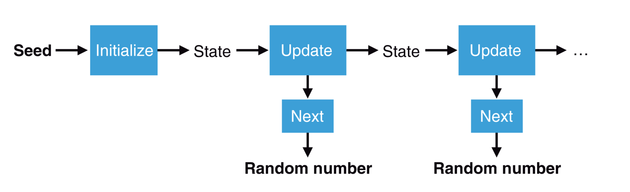
Cryptographically secure PRNGs usually tend to exhibit the following properties:
-
Deterministic
In this context, this means that once you know the initial seed, and how the next number is generated (i.e., you know how the PRNG algorithm works), then you can generate the entire sequence. This implies that using the same initial seed will always give you the same sequence of numbers.
-
Indistinguishable from random
You should not be able to distinguish a number that is randomly generated by a PRNG, and a number that is chosen uniformly at random from the same set. Consequently, observing the random numbers generated alone shouldn’t allow anyone to recover the internal state of the PRNG.
Additional security properties
A PRNG has forward secrecy if an attacker learning the state (by getting in your computer at some point in time, for example) doesn’t allow the PRNG to retrieve previously generated random numbers.
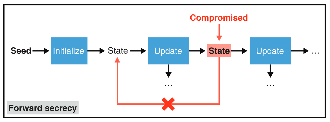
Obtaining the state of a PRNG means that you can determine all future pseudorandom numbers that it will generate. To prevent this, some PRNGs have mechanisms to “heal” themselves periodically (in case there was a compromise). This healing can be achieved by reinjecting (or re-seeding) new entropy after a PRNG was already seeded. This property is called backward secrecy.
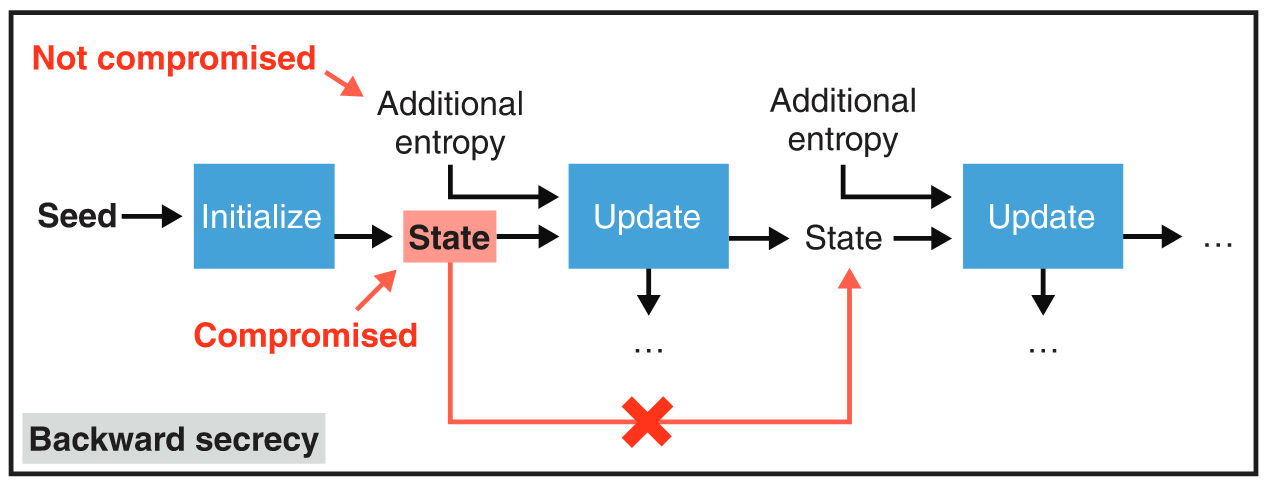
PRNGs can be extremely fast and are considered safe methods to generate large numbers of random values for cryptographic purposes if properly seeded. Using a predictable number or a number that is too small is obviously not a secure way to seed a PRNG. This effectively means that we have secure cryptographic ways for quickly stretching a secret of appropriate size to billions of other secret keys.
Using randomness in practice
As a summary, an operating system needs the following things in order to provide “cryptographically secure” random numbers:
-
Sources of entropy
These are ways for the OS to obtain raw randomness from unpredictable physical phenomena like the temperature of the device or your mouse movements.
-
Cleaning and mixing
A single source of entropy by itself may be a rather poor source of randomness, so the OS cleans up and mixes a number of sources together to produce a better, more consistent quality of randomness.
-
PRNGs
In order to optimize the speed of random number generation, the OS uses a PRNG seeded from a single, uniformly random value to efficiently generate random numbers.
More often than not, the operating system comes with an interface that abstracts away the fine details into simplified functions for developers to generate a random number just by issuing a system call.
The way operating systems implement and provide access to this
functionality obviously differ from one OS to another. Linux uses a PRNG
that’s based on the ChaCha20 stream cipher, and following the
“everything is a file” metaphor, such an interface is available as a
special file called /dev/urandom. For instance, one can read \(128\)
bytes from the terminal using the dd command-line utility:
brian@thonkpad ~/classes/csci184.03
% dd if=/dev/urandom bs=128 count=1 2> /dev/null | xxd -p
36041307dcb45514899cd0a5765921f07043ffeeeb23d6d9dbd79f18337e
9d1b2bad022bd4b4eba667faf925c7182b556ef2cd4cfc29d75191dfc453
d46dc59570137b8adae09ffcf1af521b9195b68145e5969b76cfe58beea2
7a7ff4ab612e92d365fc55465a7277531b2e90cc8146d486d37f037e547c
e0bc1515cebf520e
One problem with /dev/urandom in particular is that it might not
provide enough entropy (its numbers won’t be random enough) if used too
early after booting the device.
To avoid “low-level” issues like this, most programming languages
provide methods and functions for random number generation. In Python,
there are two modules dedicated for this purpose, one called random,1
and the other called secrets.2 The functions provided in random use a
PRNG called the Mersenne
Twister, which is not
by any means considered cryptographically secure (the Python docs even
state that random is designed for modeling and simulation). On the
other hand, secrets actually rely on the operating system’s random
number generator, which is guaranteed to produce cryptographically
strong random numbers suitable for managing sensitive data like
passwords and tokens.
References
- Wong, David. 2021. Real-World Cryptography. Manning Publications.
Stream ciphers
Relevant readings: Aumasson ch. 5
Introducing stream ciphers
Stream ciphers take two values: a key and a nonce (which stands for “number used only once”),1 and produce a pseudorandom stream of bits called the keystream. The key should be secret and is usually \(128\) or \(256\) bits. The nonce doesn’t have to be secret, but it should be unique for each key and is usually between \(64\) and \(128\) bits.
Encryption and decryption work similarly to the one-time pad: the keystream is XOR’ed with the plaintext to encrypt it, and the ciphertext is XOR’ed with the keystream to decrypt it. More concretely, a stream cipher produces a keystream \(\textit{KS} = \textsf{SC}(K, N)\) given a secret key \(K\) and a public nonce \(N\), encrypts as \(C = P \oplus \textit{KS}\), and decrypts as \(P = C \oplus \textit{KS}\).
Stateful and counter-based stream ciphers
Stream ciphers generally belong into two main types: stateful and counter-based.
From the name itself, a stateful stream cipher uses an internal state to facilitate the generation of the keystream. It sets up the initial state using the key and the nonce, and then uses the update function to update the state and produce a keystream bit, as shown in Figure 1.
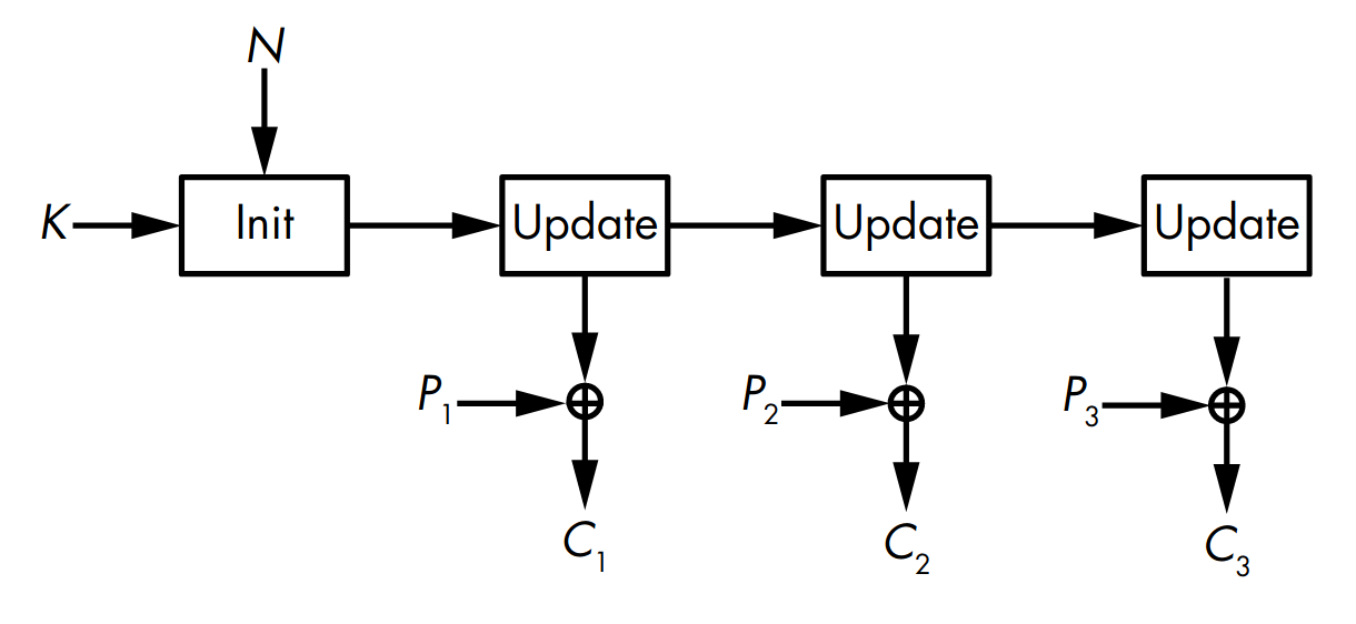
A counter-based stream cipher produces chunks of keystream from a key, a nonce, and a counter value, as shown in Figure 2.
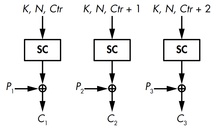
Hardware and software implementations
A cipher’s hardware implementation refers to the dedicated electronic circuit that implements the cryptographic algorithm. These usually come in the form of application-specific integrated circuits (ASICs), programmable logic devices (PLDs), and field-programmable gate arrays (FPGAs). As such, these can’t be used for anything else other than the cryptographic algorithm itself. On the other hand, a software implementation is just a set of instructions to be executed by a microprocessor.
A notable difference between hardware and software implementations is that hardware-based ciphers deal with bits, while software-based ciphers deal with bytes or words (\(32\) or \(64\) bits depending on the processor).
Feedback shift registers
Feedback shift registers (FSRs) are the simplest hardware stream ciphers. Under the hood they are just an array of bits equipped with a feedback function.
Let \(R_0\) be the initial value of the FSR. Then the next state \(R_1\) is defined as \(R_0\) left-shifted by \(1\) bit. The bit that got pushed out the register is returned as output, while the newly emptied position is filled with \(f(R_0)\).
This process is then repeated for the next state values. Given the current state of the FSR \(R_t\), the next state \(R_{t+1}\) can be computed using the following recurrence: $$R_{t+1} = (R_t \shl 1) \BitOr f(R_t)$$ where \(\BitOr\) is the bitwise OR operator and \(\shl\) is the left shift operator.
Suppose we have a \(4\)-bit FSR, whose feedback function \(f\) takes
the XOR of all four bits, and the state is initialized as 1100. To get
the next state, we shift the bits to the left and then set the rightmost
bit as
\(f(\texttt{1000}) = \texttt{1} \oplus \texttt{0} \oplus \texttt{0} \oplus \texttt{0} = \texttt{1}\).
Thus the state becomes 0001 and it outputs 1.
We repeat this process three more times to produce three more keystream
bits, which gives the state values 0011, 0110, and 1100.
Notice that we return to our initial state 1100 after five iterations,
so we say that \(5\) is the period of the FSR. Naturally we would
want a longer period and less repeating patterns for better security.
Linear feedback shift registers
Linear feedback shift registers (FSRs) are FSRs with a linear feedback function. Usually such functions involve XOR’ing some bits of the state, just like the feedback function presented in the previous example. We refer to the bits that influence the input as taps.
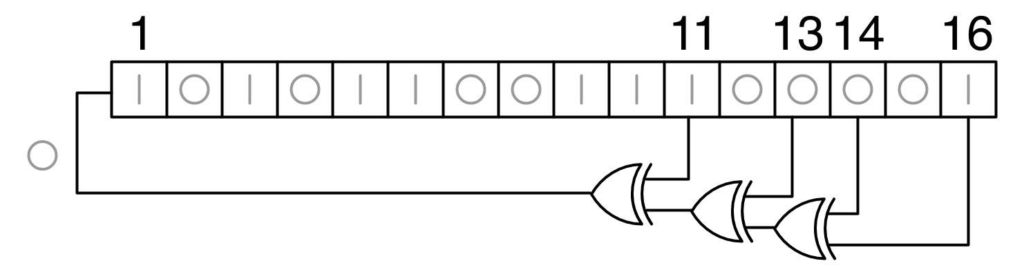
LFSRs use the arithmetic over the finite field \(\FF_{2^n}\), represented as polynomials whose coefficients are either \(0\) or \(1\). The feedback function then is a polynomial expression that encodes which bits are used as taps, specifically for an \(n\)-bit LFSR uses the feedback polynomial $$\sum_{i=0}^n x^i = x^n + \cdots + x^2 + x + 1$$ where the term \(x^i\) is only included if the \(i\)th bit is a tap. For example, the LFSR shown in Figure 3 uses bits \(11\), \(13\), \(14\), and \(16\) as taps, so its feedback polynomial is $$x^{16} + x^{14} + x^{13} + x^{11} + 1.$$ The “\(1\)” in the polynomial doesn’t actually correspond to a tap, but rather, it corresponds to the input to the first bit. As a rule of thumb, the feedback polynomial of an \(n\)-bit LFSR always contains a “\(1\)” and an “\(x^n\)” term.
Every polynomial \(f(x)\) with coefficients in \(\FF_2\) having \(f(0) = 1\) divides \(x^m + 1\) for some \(m\). The smallest \(m\) for which this is true is called the period of \(f(x)\). It’s also helpful to know that an irreducible polynomial of degree \(n\) has a period which divides \(2^n - 1\), and an irreducible polynomial of degree \(n\) whose period is \(2^n - 1\) is called a primitive polynomial.2 To find a suitable feedback polynomial for an \(n\)-bit LFSR, we can use the following theorem (which we won’t prove here):
An \(n\)-bit LFSR is maximal iff its feedback polynomial is a primitive polynomial of degree \(n\) over \(\FF_{2}\).
-
\(x^4 + x^3 + x^2 + 1\) is not irreducible over \(\FF_2\) since we can factor it as \((x+1)(x^3+x+1)\).
-
\(x^4 + x^3 + x^2 + x + 1\) is irreducible over \(\FF_2\) since it has no linear factors. But \(x^5 + 1 = (x+1) (x^4 + x^3 + x^2 + x + 1)\) so it has period \(5\), and \(5 \ne 2^4 - 1 = 15\) so it is not a primitive polynomial.
-
\(x^4 + x^3 + 1\) is irreducible over \(\FF_2\). Thus it has a period which divides \(2^4-1 = 15\); its divisors are \(1, 3, 5, 15\). Since the period must be greater than \(4\), there are two possible values: \(5\) and \(15\). We try each value and get the following: $$\begin{align} x^5 + 1 &= (x+1) (x^4 + x^3 + 1) + (x^3+x) \\ x^{15} + 1 &= (x^{11} + x^{10} + x^9 + x^8 + x^6 + x^4 + x^3 + 1) (x^4 + x^3 + 1) \end{align}$$
Therefore \(x^4 + x^3 + 1\) has period \(15\), so it is a primitive polynomial.
If we want to achieve the maximal LFSR, these conditions are then necessary (but not sufficient):
-
There must be an even number of taps.
-
The set of taps are relatively prime to each other, meaning if we have the set of taps \(\Set{t_1, \ldots, t_m}\) then \(\gcd(t_1, \ldots, t_m) = 1\).
SageMath has bulit-in functionality for constructing LFSRs:
FF = GF(2)
P.<x> = PolynomialRing(FF)
lfsr = LFSRCryptosystem(FF)
# cast each element in the list as elements of GF(2)
init_state = list(map(FF, [0,1,1,0,1,1,0,1,0,1]))
fb = x^10 + x^8 + x^5 + x^4 + 1
# if fb is primitive then our LFSR is maximal
fb.is_primitive()    # ==> True
e = lfsr((fb, init_state))
# generate 32 bytes worth of zeros
m = e.domain().encoding('\x00'*32)
# output first 32 bytes of the keystream
e(m)
Using an LFSR as a stream cipher on its own is insecure, as an attacker only needs \(2n\) output bits to recover the initial state of an \(n\)-bit LFSR and allow them to determine the previous and future bits. This is carried out using the Berlekamp–Massey algorithm that solves the equations defined by the LFSR’s mathematical structure to recovers the initial state and the feedback polynomial. You can even do this attack using SageMath:
# yoinked somewhere in the middle
ks = [0,0,0,0,1,1,1,1,0,0,0,0,0,1,1,0,0,1,1,1]
from sage.matrix.berlekamp_massey import berlekamp_massey
berlekamp_massey(list(map(GF(2), ks)))
It is important to note that LFSRs are not cryptographically secure because they are linear, and so output bits and initial state bits can be recovered using techniques from linear algebra.3 To work around this problem, stuff such as nonlinearity is introduced to strengthen LFSRs.
A5/1
A5/1 is a stream cipher that was used to encrypt voice communications in the GSM mobile standard.
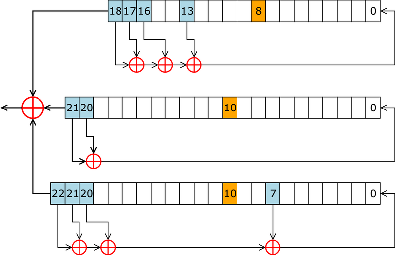
It uses three LFSRs with \(19\), \(22\), and \(23\) bits (as shown in Figure 4) where the feedback polynomials for each as follows: $$\begin{align} &x^{19} + x^{18} + x^{17} + x^{14} + 1 \\ &x^{22} + x^{21} + 1 \\ &x^{23} + x^{22} + x^{21} + x^8 + 1\end{align}$$
Unlike the typical LFSRs, its update mechanism is different. Instead of updating all three LFSRs at each clock cycle, the designers of A5/1 added a clocking rule that does the following:
-
Check the value of the ninth bit of LFSR 1, the \(11\)th bit of LFSR 2, and the \(11\)th bit of LFSR 3, called the clocking bits. Of those three bits, either all have the same value (
1or0) or exactly two have the same value. -
Clock the registers whose clocking bits are equal to the majority value,
0or1. Either two or three LFSRs are clocked at each update.
A5/1 is vulnerable to known-plaintext attacks since these attacks also recover the 64-bit initial state of the system (i.e., all of the initial states of the three LFSRs), which reveals the \(22\)-bit nonce and the \(64\)-bit key used by GSM.
By 2010, it became possible to decrypt calls encrypted with A5/1 in near-real time, so telcos tried to mitigate such attacks, and thus a push to come up with a real solution. Later standards such as 3G and LTE ditched A5/1 altogether.
RC4
RC4 is a stream cipher designed by Ron Rivest in 1987. Unlike LFSRs, RC4 is more suited to be implemented in software as it does not use any other operations than addition and swapping. Originally a trade secret, the source code of RC4 was anonymously posted in 1994, and then was leaked and reverse-engineered within days.4 RC4 was notably used in the very first Wi-Fi encryption protocol called Wired Equivalent Privacy (WEP)5 and in the Transport Layer Security (TLS) protocol. We will see later why RC4 is no longer secure enough for most applications today.
How RC4 works
RC4 maintains an internal state, which consists of an array \(S\) representing one of the possible permutations of all \(256\) bytes, initially set to \(S[0] = 0\), \(S[1] = 1\), …, \(S[255] = 255\). Using a key scheduling algorithm, \(S\) is then initialized based on the supplied key \(K\).
KSA(\(K\)):
1: for \(i :=0 \ \textbf{to}\ 255\)
2: \(S[i] :=i\)
3: \(j :=0\)
4: for \(i :=0 \ \textbf{to}\ 255\)
5: \(j :=(j + S[i] + K[i \bmod K.\textit{length}]) \bmod 256\)
6: swap \(S[i]\) with \(S[j]\)
The keystream, which is of the same length as the plaintext, is then generated using a pseudorandom generator.
PRG(\(m\)):
1: \(i :=0\)
2: \(j :=0\)
3: for \(b :=0 \ \textbf{to}\ m-1\)
4: \(i :=(i+1) \bmod 256\)
5: \(j :=(j+ S[i]) \bmod 256\)
6: swap \(S[i]\) with \(S[j]\)
7: \(\textit{KS}[b] :=S[(S[i] + S[j]) \bmod 256]\)
Suppose we have an all-zero \(128\)-bit as the key. Running the key scheduling algorithm, \(S\) would now become $$[0, 35, 3, 43, 9, 11, 65, 229, \ldots, 233, 169, 117, 184, 31, 39]$$ If we want to generate a \(10\)-byte keystream, running the pseudorandom generator yields: $$[222, 24, 137, 65, 163, 55, 93, 58, 138, 6].$$
Although many people back then considered RC4 “too simple to be broken,” it didn’t stop them from finding exploitable weaknesses.
RC4 as used in WEP
WEP was the very first security protocol for Wi-Fi since the IEEE 802.11 standard was first released in 1997, and for some time this was the only form of security available for Wi-Fi routers supporting the 802.11a and 802.11b standards.
Within the implementation of WEP, RC4 was used as its pseudorandom generator. Unlike most stream ciphers, RC4 did not take a nonce as input, so the workaround was to concatenate it with the secret key, and then feed that to RC4 as the seed. That is, the key \(K\) is appended to the \(24\)-bit nonce \(N\), the actual RC4 key used is \(N \mathrel{\hspace{1pt}||\hspace{1pt}}K\). As a result, the \(128\)-bit WEP protocol actually offers only \(104\)-bit security, and the weaker \(64\)-bit WEP actually offers only \(40\)-bit security!
But that’s not the only problem about WEP:
-
Since the nonce is only \(24\) bits long, there are \(2^{24} = 16777216\) possible choices. This means it only took a few megabytes’ worth of traffic until two packets are encrypted with the same nonce. The attacker can intercept these two packets and do a known-plaintext attack to recover the other message.
-
Combining the nonce and key in this fashion helps recover the key. Since the nonce is publicly-viewable, it is possible to determine the value of \(S\) after three iterations of the key scheduling algorithm.
These weaknesses allow for known-plaintext and chosen-plaintext attacks
against WEP. Not only these attacks are possible in theory, these are
very much possible in practice (e.g., tools like aircrack-ng implement
the entire attack). Further refinements have lessened the number of
captured packets needed to carry out the attack.6
Thus WEP was eventually deprecated in 2004, by which Wi-Fi Protected Access (WPA) and WPA2 were made available as replacements with the ratification of the full 802.11i standard.
Segue: Why did old schemes use keys that are too short?
Believe it or not, the main reason was not because of the limitations of technology at that time.
Here’s a quick history of cryptography policy, at least in the United States. In the Cold War era, cryptography was almost exclusively used by the military, so encryption technology (which eventually included cryptography software) was included into the United States Munitions List in 1954, which put basically everything that uses cryptography in the same league as missiles, bombs, grenades, and flamethrowers. This means the export of cryptography outside the US was severely restricted and heavily regulated for reasons involving national security.7
As cryptography became increasingly widespread in non-military applications, namely for commercial usage, these restrictions became problematic. For example, Netscape released two versions of its browser: one for the US market that supported “full-size” keys (such as \(128\)-bit RC4), and another one for the rest of the world that used reduced key lengths (such as \(40\)-bit RC4). This was also the case for WEP, where two versions are released, namely WEP-40 and WEP-104.
It wasn’t until the late 1990s when these export restrictions were gradually eased, due to legal challenges brought by privacy advocates, though some restrictions still remain today.8
Stream ciphers gone wrong
Nonce reuse
The most common mistake involving stream ciphers is when a nonce is reused with the same key. This is similar to when you reuse the key in a one-time pad: once you have two ciphertexts, you can XOR them together to get the XOR of the two plaintexts, where the identical keystreams cancel each other out in the process.
Broken RC4 implementation
Here’s yet another reason why you don’t implement cryptographic algorithms from scratch. If you were to implement RC4 on your own, there’s a chance that you an already weak cipher even weaker!
Typically, you would implement a swap operation involving \(S[i]\) and \(S[j]\) by using a temporary variable like this:
1: \(\textit{temp} :=S[i]\)
2: \(S[i] :=S[j]\)
3: \(S[j] :=\textit{temp}\)
This is fine, but if space is at a premium you would want to avoid using additional variables as much as possible. Another way that some programmers do is to use a piece of black magic called an XOR swap:
1: \(x :=x \oplus y\)
2: \(y :=x \oplus y\)
3: \(x :=x \oplus y\)
This works since the second line sets \(y\) to \((x \oplus y) \oplus y = x\) and the third line sets \(x\) to \((x \oplus y) \oplus (x \oplus y \oplus y) = y\).
Now take a moment to see what could go wrong if we do the XOR swap for \(S[i]\) and \(S[j]\) (try it by plugging your own values of \(i\) and \(j\)):
1: \(S[i] :=S[i] \oplus S[j]\)
2: \(S[j] :=S[i] \oplus S[j]\)
3: \(S[i] :=S[i] \oplus S[j]\)
What if \(i\) is equal to \(j\)? Instead of leaving the state unchanged, the XOR swap will set \(S[i]\) to \(S[i] \oplus S[i] = 0\), so a byte of the state will be set to zero each time \(i\) equals \(j\) in the key scheduling algorithm and in the pseudorandom generator. Repeat this enough and this would eventually lead to all-zero state and thus to an all-zero keystream. Yikes!
The moral of the story here is to not fix what’s not broken (i.e., do not over-optimize your implementation) and that sometimes the best solution is the simplest one.
References
- Aumasson, Jean-Philippe. 2017. Serious Cryptography: A Practical Introduction to Modern Encryption. No Starch Press.
In the context of stream ciphers, a nonce is also called an initialization vector (IV).
This is pretty similar to the notion of generators in group theory.
For example, Gauss–Jordan elimination works in any field, whether \(\RR\) or \(\FF_2\).
Naturally, this led to a “chilling effect” that prevented academic cryptographers from publishing their research, because doing so would violate these export laws.
Block ciphers
Relevant readings: Aumasson ch. 4
What is a block cipher?
A block cipher is a type of cipher that combines a core algorithm working on blocks of data with a mode of operation, or a technique to process sequences of data blocks. More formally, a block cipher consists of two deterministic algorithms:
-
The encryption algorithm Enc takes as input a key \(k\) and a plaintext message \(m \in \Set{\texttt{0}, \texttt{1}}^*\), and outputs a ciphertext \(c\).
-
The decryption algorithm Dec takes as input a key \(k\) and a ciphertext \(c\), and outputs a message \(m \in \Set{\texttt{0}, \texttt{1}}^*\).
Usually Dec is defined as the inverse of Enc, so their corresponding implementations are similar.
Block cipher constructions
Though there are lot of block ciphers in use today, there’s only a handful of ways to construct one.
Rounds
A block cipher works by computing a sequence of rounds. A single round in a block cipher does a basic transformation that is easy to specify and implement. Putting these rounds together, we form the block cipher’s algorithm.
For example, a block cipher with three rounds encrypts a plaintext by computing \(C \gets R_3(R_2(R_1(P)))\), where the rounds are \(R_1\), \(R_2\), and \(R_3\), and \(P\) is the plaintext. The rounds must have an inverse so that it is possible to decrypt the ciphertext by computing \(P \gets R_1^{-1}(R_2^{-1}(R_3^{-1}(C)))\).
These round functions use the same algorithm, but they take an additional parameter called the round key, which means that two round functions with two distinct round keys will behave differently, and therefore will produce distinct outputs if fed with the same input.
Substitution–permutation networks
For a cipher to be considered secure, it needs to have two properties: confusion and diffusion. Confusion obscures the relationship between the key and the ciphertext as much as possible using complex transformations, and diffusion means that these transformations depend equally on all bits of the input. In the design of block ciphers, confusion is provided by substitution operations while diffusion is provided by permutation operations; when combined together they form a substitution–permutation network (SPN).
Substitution operations are done using substitution boxes, or S-boxes for short. An S-box substitutes a small block of input bits with another block of output bits using some sort of a lookup table.
One of the S-boxes used in the Data Encryption Standard (DES), namely \(S_5\), maps a \(6\)-bit input into a \(4\)-bit output as defined in the following table:
| 0 | 1 | 2 | 3 | 4 | 5 | 6 | 7 | 8 | 9 | 10 | 11 | 12 | 13 | 14 | 15 | |
| 2 | 12 | 4 | 1 | 7 | 10 | 11 | 6 | 8 | 5 | 3 | 15 | 13 | 0 | 14 | 9 | |
| 1 | 14 | 11 | 2 | 12 | 4 | 7 | 13 | 1 | 5 | 0 | 15 | 10 | 3 | 9 | 8 | 6 |
| 2 | 4 | 2 | 1 | 11 | 10 | 13 | 7 | 8 | 15 | 9 | 12 | 5 | 6 | 3 | 0 | 14 |
| 3 | 11 | 8 | 12 | 7 | 1 | 14 | 2 | 13 | 6 | 15 | 0 | 9 | 10 | 4 | 5 | 3 |
To see how this works, say we have an input 011011. It has outer bits
01 and inner bits 1101, which are \(1\) and \(13\) in decimal
respectively. The \(4\)-bit output is found by selecting the \(1\)st
row and the \(13\)th column, so the output is \(9\) or 1001 in
this case.
Permutation operations can be as simple as swapping or shuffling the bits. Some ciphers use linear algebra to permute the bits, like using a series of multiplication operations with fixed values and adding them up. Such linear algebra operations can quickly create dependencies between all the bits within a cipher and thus ensure strong diffusion.
Feistel networks
Feistel networks were first used in IBM’s block cipher called Lucifer, designed by Horst Feistel in the 1970s. Here’s a high-level description of how it works:
-
Split the \(64\)-bit block into \(32\)-bit halves \(L_0\) and \(R_0\).
-
Set \(L_1\) to \(L_0 \oplus f(R_0)\).
-
Swap the values of \(L_1\) and \(R_1\).
-
Repeat steps 2–3 fifteen times to get the values for \(L_2, \ldots, L_{16}\) and \(R_2, \ldots, R_{16}\).
-
Merge \(L_{16}\) and \(R_{16}\) into the \(64\)-bit output block.
Figure 1 visualizes this process.
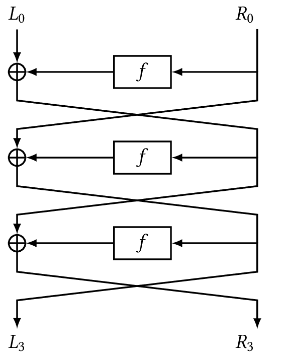
The \(f\) functions each correspond to a substitution–permutation round, so they also take a round key \(K_i\). More precisely, \(f\) can be either a pseudorandom permutation or a pseudorandom function. But in a Feistel network, that difference doesn’t matter as long as \(f\) is cryptographically strong.
The number of rounds in a Feistel network depends on how strong \(f\) is. If it is strong enough, then four rounds may be enough, but real block ciphers use a lot more rounds to defend against any potential weaknesses in \(f\). DES, for example, performs \(16\) rounds.
The Advanced Encryption Standard (AES)
The Advanced Encryption Standard (AES) is the most widely-used block cipher ever. Its predecessor the Data Encryption Standard (DES), which was published in 1977, was broken in 1999 after a brute-force attack was demonstrated to be feasible in practice. Soon after, the National Institute of Standards and Technology (NIST) announced the “AES competition” to choose a successor to DES. In 2000, NIST selected a new cipher called Rijndael (pronounced like “rain-dull”) as the replacement for DES and it was standardized as AES, at which point it became the world’s de facto encryption standard.1
The internals of AES
AES processes blocks of \(128\) bits using a secret key of \(128\), \(192\), or \(256\) bits, and unlike other ciphers, AES deals with bytes. A \(16\)-byte plaintext is represented as a \(4 \times 4\) matrix (or 2D array) of bytes \(s_0, s_1, \ldots, s_{15}\): $$\begin{bmatrix} s_0 & s_1 & s_2 & s_3 \\ s_4 & s_5 & s_6 & s_7 \\ s_8 & s_9 & s_{10} & s_{11} \\ s_{12} & s_{13} & s_{14} & s_{15} \end{bmatrix}$$ More precisely, these bytes correspond to elements in the finite field of \(256\) elements \(\FF_{256}\) defined by the polynomial ring \(\FF_2[x]/\gen{x^8+x^4+x^3+x+1}\). The encryption process would then be transforming the bytes, columns, and rows of this matrix, which is possible since AES uses an SPN structure like the one shown in Figure 2.
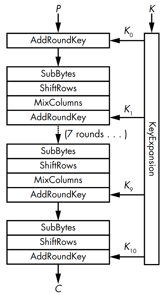
The building blocks of an AES round are:
AddRoundKey
XOR’s a round key to the internal state.
SubBytes
Replaces each byte \((s_0, s_1,\ldots, s_{15})\) with another byte
according to an S-box. In this case, the S-box is a lookup table of
\(256\) elements.
ShiftRows
Shifts the \(i\)th row of \(i\) positions, for \(i\) ranging from
\(0\) to \(3\). $$\begin{bmatrix}
s_0 & s_4 & s_8 & s_{12} \\
s_1 & s_5 & s_9 & s_{13} \\
s_2 & s_6 & s_{10} & s_{14} \\
s_3 & s_7 & s_{11} & s_{15}
\end{bmatrix}
\xrightarrow[\textsf{ShiftRows}]{}
\begin{bmatrix}
s_0 & s_4 & s_8 & s_{12} \\
s_5 & s_9 & s_{13} & s_1 \\
s_{10} & s_{14} & s_2 & s_6 \\
s_{15} & s_3 & s_7 & s_{11}
\end{bmatrix}$$
MixColumns
Applies the same linear transformation to each of the four columns of
the state. This is accomplished using matrix multiplication over
\(\FF_{256}\) where each column is multiplied by a constant square
matrix defined by $$\begin{bmatrix}
\texttt{02} & \texttt{03} & \texttt{01} & \texttt{01} \\
\texttt{01} & \texttt{02} & \texttt{03} & \texttt{01} \\
\texttt{01} & \texttt{01} & \texttt{02} & \texttt{03} \\
\texttt{03} & \texttt{01} & \texttt{01} & \texttt{02}
\end{bmatrix}$$
These operations also have inverse counterparts for the sake of decryption, namely AddRoundKey (self-inverse), InvSubBytes, InvShiftRows, and InvMixColumns.
The key scheduling algorithm is provided by the function called KeyExpansion that creates \(11\) round keys \(K_0, K_1, \ldots, K_{10}\) of \(16\) bytes each from the \(16\)-byte key. One important property of KeyExpansion is that given any round key, \(K_i\), an attacker can determine all other round keys as well as the main key, by reversing the algorithm.
Implementing AES
Unlike DES, which was originally designed to be implemented with integrated circuits, AES is designed with mainstream CPUs in mind so it is fast in software. Modern x86 processors since 2010 now have built-in instructions for encrypting and decrypting with AES, called the AES New Instructions (AES-NI), as an extension to the x86 instruction set. Most likely your computer’s CPU already supports it:
brian@thonkpad ~/classes/csci184.03
% cat /proc/cpuinfo | grep aes -m 1
flags           : fpu vme de pse tsc msr pae mce cx8 apic sep mtrr pge mca cmov pat
pse36 clflush dts acpi mmx fxsr sse sse2 ss ht tm pbe syscall nx pdpe1gb rdtscp lm
constant_tsc art arch_perfmon pebs bts rep_good nopl xtopology nonstop_tsc cpuid
aperfmperf tsc_known_freq pni pclmulqdq dtes64 monitor ds_cpl vmx smx est tm2 ssse3
sdbg fma cx16 xtpr pdcm pcid sse4_1 sse4_2 x2apic movbe popcnt tsc_deadline_timer aes
xsave avx f16c rdrand lahf_lm abm 3dnowprefetch cpuid_fault epb invpcid_single ssbd
ibrs ibpb stibp ibrs_enhanced tpr_shadow vnmi flexpriority ept vpid ept_ad fsgsbase
tsc_adjust bmi1 avx2 smep bmi2 erms invpcid rdseed adx smap clflushopt clwb intel_pt
sha_ni xsaveopt xsavec xgetbv1 xsaves split_lock_detect avx_vnni dtherm ida arat pln
pts hwp hwp_notify hwp_act_window hwp_epp hwp_pkg_req hfi umip pku ospke waitpkg gfni
vaes vpclmulqdq rdpid movdiri movdir64b fsrm md_clear serialize arch_lbr ibt flush_l1d
arch_capabilities
Instead of manually coding an AES round as a sequence of assembly
instructions, you can simply use the AESENC instruction and the CPU
will do the round for you.
PXOR       %xmm5,  %xmm0    ; XOR the first round key
AESENC     %xmm6,  %xmm0
AESENC     %xmm7,  %xmm0
AESENC     %xmm8,  %xmm0
AESENC     %xmm9,  %xmm0
AESENC     %xmm10, %xmm0
AESENC     %xmm11, %xmm0
AESENC     %xmm12, %xmm0
AESENC     %xmm13, %xmm0
AESENC     %xmm14, %xmm0
AESENCLAST %xmm15, %xmm0    ; last round of AES
When the first x86 processors were introduced in 1978, they only have
fourteen \(16\)-bit registers, four of which are general-purpose
registers called ax, bx, cx, and dx. Each of the can be accessed
as two separate bytes (as “high” or “low” bytes), so ah corresponds to
ax’s high byte while al corresponds to ax’s low byte.
Over the years, the word size of x86 has been extended twice (the first
one was to \(32\) bits, and the second one was to \(64\) bits), and
thus also came extended registers. A \(32\)-bit register is prefixed
with an “e” so the ax register corresponds to the lowest \(16\)
bits of the eax register. Likewise, a \(64\)-bit register is
prefixed with an “r” so we have rax, rbx, and so on.
More recently, extensions to x86 such as Streaming SIMD Extensions
(SSE) and Advanced Vector Extensions (AVX) introduced even larger
registers. SSE provides \(128\)-bit registers named xmm0–xmm15,
and AVX provides \(256\)-bit registers named ymm0–ymm15 and
\(512\)-bit registers named zmm0–zmm31 from AVX-512.
Modes of operation
In this section, we present the main modes of operation used by block ciphers.
Electronic codebook (ECB)
The simplest mode is the electronic codebook (ECB). All it does is it takes blocks of plaintexts \(P_1, \ldots, P_n\) and these blocks are encrypted separately as \(C_i \gets \Enc{k}{P_i}\) for all \(i = 1, \ldots, n\), as shown in Figure 3.
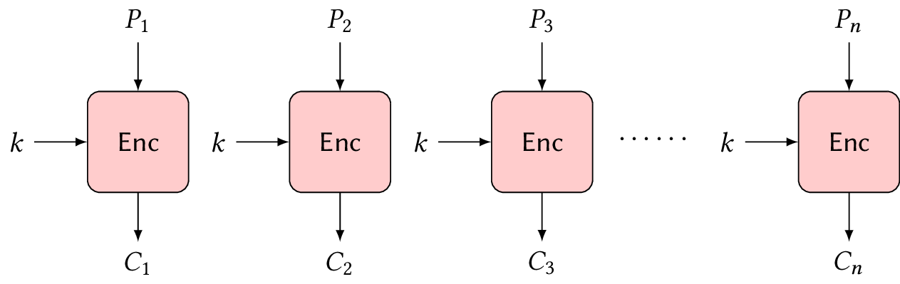
It also turns out to be really insecure, and here’s why. I have an image of Tux, the Linux mascot, encrypted with a block cipher in ECB mode, and you can see the result of the encryption in Figure 4. As you can see, the patterns in the image still persist even after encryption even though the actual pixel values remain encrypted, so ECB encryption just gives you the same image but with different colors.
This is one of the iconic images in the cryptography and infosec community, as everyone who has some working knowledge of cryptography will surely have recognized this image. So if anyone asks why we shouldn’t use ECB mode, we just show them this image.2 If there’s anything to take away from this course, it’s this: never use ECB mode, ever!
Another problem with ECB mode is that it expects blocks to have the same size, so it will have trouble encrypting plaintext that does not cleanly divide into blocks of equal size unless some kind of padding is used.
Cipher block chaining (CBC)
Cipher block chaining (CBC) works like ECB, but it takes a random initialization vector (IV) which is XOR’ed with the first plaintext block, which is then fed into the encryption algorithm, and the output ciphertext block is also XOR’ed into the next plaintext block, and so on. That is, CBC encrypts the \(i\)th block as \(C_i \gets \Enc{k}{P_i \oplus C_{i-1}}\), where \(C_{i-1}\) is the previous ciphertext block. For \(C_1\), it takes the IV instead since there’s no previous ciphertext block to use.
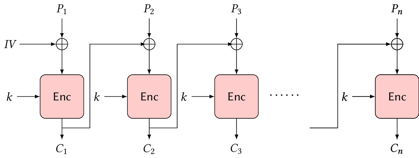
As a result, each ciphertext block is now dependent on all the previous blocks, so identical plaintext blocks won’t encrypt to identical ciphertext blocks.
Dealing with arbitrary-length data
Most of real-life data don’t split evenly into blocks. What if, for example, we want to encrypt a \(201\)-byte plaintext with AES-CBC when blocks are \(16\) bytes? What do we do with the leftover \(9\) bytes? There are two ways to deal with this problem:
-
Padding
Make the ciphertext a bit longer than the plaintext.
-
Ciphertext stealing
Produce a ciphertext of the same length as the plaintext.
Padding appends extra bytes at the end of the leftover block to fill a complete block. One such padding scheme is the PKCS#7 standard, which is the most widely used for block ciphers. For a block size of \(16\) bytes, it works like this:
-
If there’s one byte left, pad the message with \(15\) bytes
0f(which is \(15\) in decimal). -
If there’s two bytes left, pad the message with \(14\) bytes
0e(which is \(14\) in decimal).
And so on. If the length of the original message is already a multiple
of \(16\), we pad it with a whole block of 10 (which is \(16\) in
decimal). This seems simple enough to do it in Python:
def pkcs7_pad(p, blklen=16):
    n = blklen - (len(p) % blklen)  # find number of bytes to pad
    pad = bytes([n] * n)            # generate the extra bytes
    return p + pad                  # and add it to the end
Then we try it for some arbitrary-length bytestrings:
>>> pkcs7_pad(b'This is getting padded!', 26)
b'This is getting padded!\x03\x03\x03'
>>> pkcs7_pad(b'this has 16bytes')
b'this has 16bytes\x10\x10\x10\x10\x10\x10\x10\x10\x10\x10\x10\x10\x10\x10\x10\x10'
Another method, though less popular than padding, is ciphertext stealing. Its advantage over padding is that it can deal with plaintexts of any bit length, not just bytes, and that ciphertexts are exactly the same length as plaintexts. More importantly, CBC with ciphertext stealing is resistant to padding oracle attacks (we’ll talk about this later).
Figure 4 shows the process of ciphertext stealing in CBC mode. Here, ciphertext stealing extends the last incomplete plaintext block (shown in blue) by “stealing” bits from the previous ciphertext block (shown in red), and then encrypts the resulting block. The last, incomplete ciphertext block is made up of the first blocks from the previous ciphertext block (shown in yellow); that is, the bits that have not been appended to the last plaintext block.
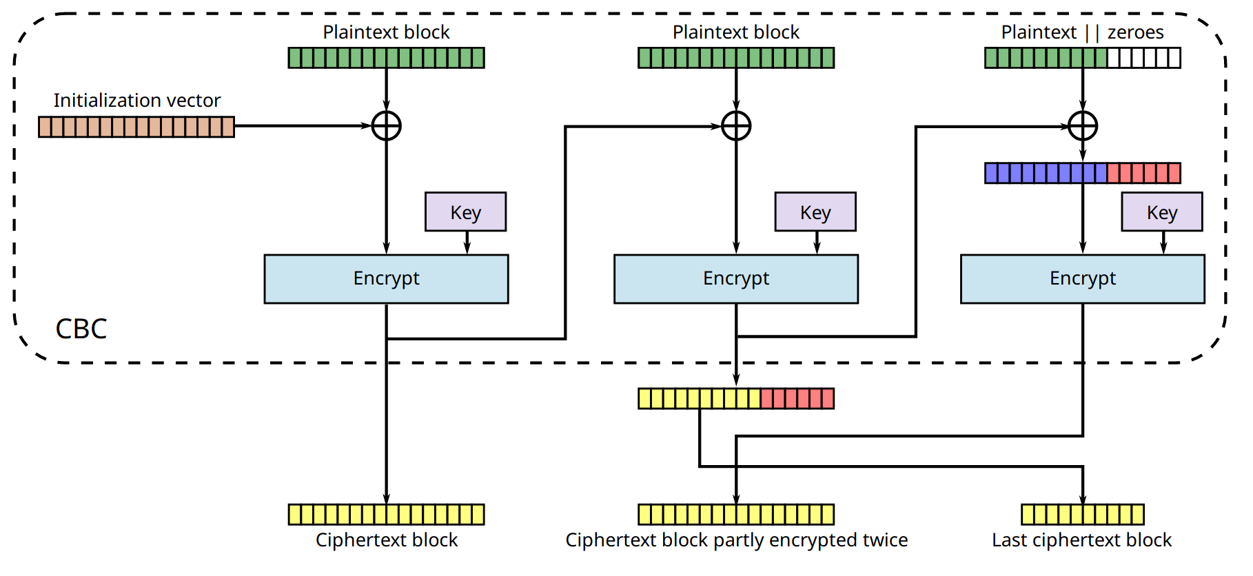
Counter (CTR) mode
The counter mode is a bit weird among other modes of operation, since this mode essentially turns a block cipher into a stream cipher. It uses the encryption algorithm of the block cipher to generate the keystream, which will then be used to actually encrypt the plaintext, as seen in Figure 5.
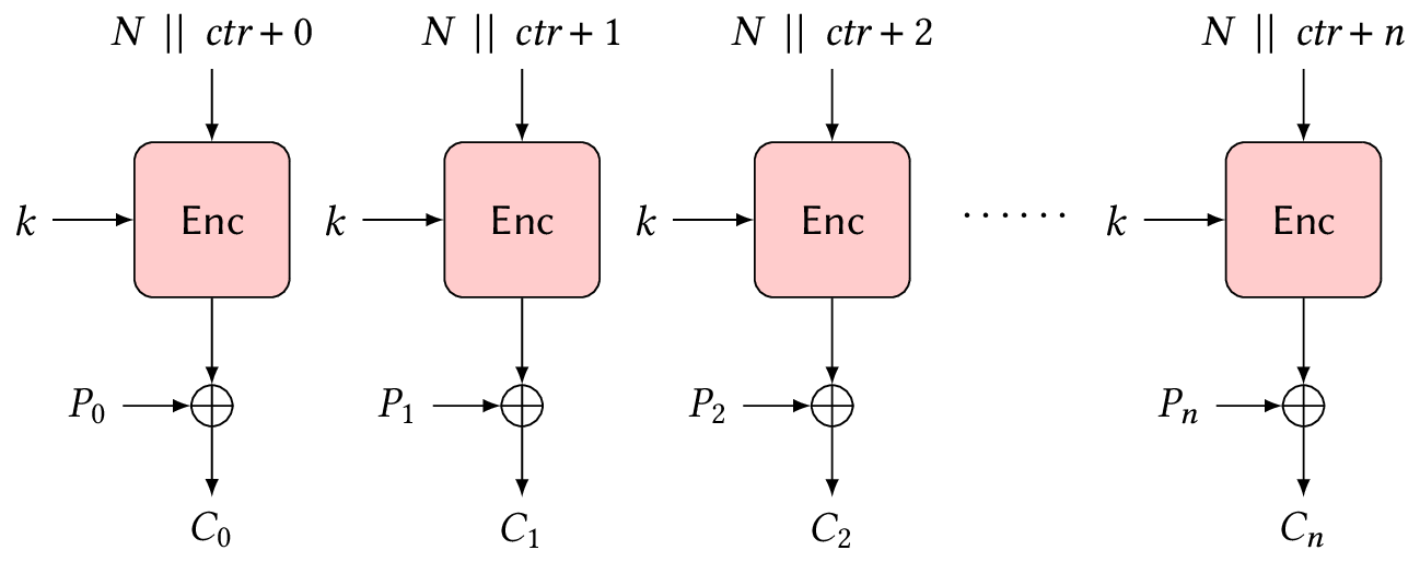
More specifically, it will encrypt blocks composed of a counter \(\textit{ctr}\), which is an integer that is incremented for each block, and a nonce \(N\), so the \(i\)th keystream block is generated by \(K_i \gets \Enc{k}{N \mathrel{\hspace{1pt}||\hspace{1pt}}\textit{ctr}+i}\) and the actual encryption is done by computing \(C_i \gets P_i \oplus K_i\) for \(i = 0, 1, \ldots, n\). Keep in mind that a nonce should not be reused to encrypt two different messages.
One advantage of CTR mode is that it can be faster than in any other mode, since it is parallelizable (i.e., each block does not depend on another in any way). Also, because CTR mode is just a glorified stream cipher, you can start encrypting the plaintext as it is being sent even without having the entire plaintext available from the start.
Other modes of operation
Aside from ECB, CBC, and CTR modes, we also have output feedback (OFB) and cipher feedback (CFB) modes, which nobody really uses in practice. There are also modes of operation for specific applications, such as Galois/Counter Mode (GCM) and counter with CBC-MAC (CCM) for authenticated encryption.
Padding oracle attacks
One of the best-known attacks in modern cryptography are padding oracle attacks. Although it was discovered in the 2002 by academic cryptographers and then ignored for some time, it was rediscovered a decade later when it was found out that SSL and web frameworks like Ruby on Rails and ASP.NET were vulnerable and by that time these attacks were demostrated to be practical.3
A padding oracle is a magical thing (usually comes in the form of a black box or an API) that can tell whether or not the padding in a CBC-encrypted ciphertext is valid. In practice, a padding oracle can be found in a service on a remote host sending error messages whenever it receives malformed ciphertexts.4 Padding oracle attacks keep track of inputs that have a valid padding and those that don’t, and exploit this information to decrypt chosen ciphertext values.
Suppose we want to decrypt the ciphertext block \(C_2\), like the one shown in Figure 6. We’re looking for some value \(X\), which is \(\Dec{k}{C_2}\), and \(P_2\), the block obtained after decrypting in CBC mode. If we pick a random block \(C_1\) and send the two-block ciphertext \(C_1 \mathrel{\hspace{1pt}||\hspace{1pt}}C_2\) to the oracle, decryption will only succeed if \(C_1 \oplus P_2\) ends with a valid padding (following the PKCS#7 standard).
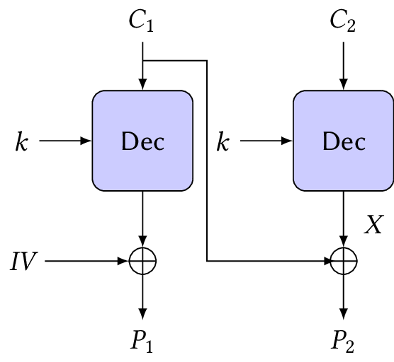
For convenience, we’ll introduce here the array notation for bytes, where \(X[0]\) is the first byte, \(X[1]\) the second, and so on. Padding oracle attacks on CBC encryption can decrypt a block \(C_2\) like this:
-
Pick a random block \(C_1\) and tweak its last byte until the padding oracle accepts the ciphertext as valid.
If the ciphertext is valid, then \(C_1[15] \oplus X[15] = \texttt{01}\).
-
Find the value \(X[14]\) by setting \(C_1[15]\) to \(X[15] \oplus \texttt{02}\) and searching for the \(C_1[14]\) that gives a correct padding.
When the padding oracle accepts the ciphertext as valid, it means we have a value for \(C_1[14]\) such that \(C_1[14] \oplus X[14] = \texttt{02}\).
-
Repeat steps 1 and 2 for all \(16\) bytes.
References
- Aumasson, Jean-Philippe. 2017. Serious Cryptography: A Practical Introduction to Modern Encryption. No Starch Press.
This is why I chose this as the icon for our Discord server, and also in the home page of this course on Canvas.
This is one of those cases when error messages can reveal too much information, like having a specific error when the padding is invalid.
Hash functions
Relevant readings: Aumasson ch. 6, Wong ch. 2
Hash functions
If you recall your CSci 30 class, a hash function maps an arbitrary-size input to a fixed-size output called a hash or digest. The usual application for these is for hash tables, a data structure that allows constant-time lookups.
Due to the pigeonhole principle,1 all hash functions are susceptible to hash collisions, where two different inputs can hash to the same output. To mitigate this, hash functions should be carefully constructed such that the probability of a hash collision occurring is as negligible as possible.
Cryptographic hash functions
Not all hash functions can be used for cryptographic applications. Checksum algorithms such as CRC-32 (as you have seen from Homework 2) are not designed with security in mind, thus making them unsuitable as cryptographic hash functions. For example, the WEP protocol from the IEEE 802.11 standard used CRC-32 as part of checking message integrity that eventually rendered it insecure, partly due to the linearity property that CRC-32 has.
A cryptographic hash function can be defined in terms of security notions, sorted from weakest to strongest:
-
Preimage resistance
Given \(y = H(x)\) for a uniform \(x\), it is infeasible for a PPT adversary to find a value \(x^\prime\) (whether equal to \(x\) or not) such that \(H(x^\prime) = y\).
In other words, \(H\) is a one-way function.
-
Second preimage resistance
Given a uniform \(x\), it is infeasible for a PPT adversary to find a second preimage \(x^\prime \ne x\) such that \(H(x^\prime) = H(x)\).
-
Collision resistance
It is infeasible for a PPT adversary to find distinct \(x, x^\prime\) such that \(H(x) = H(x^\prime)\).
Collision resistance
Since hash collisions are unavoidable, the next best thing we can do is to make generating such collisions infeasible, i.e., hard to find.
The following definition is for keyed hash functions:
A hash function, with output length \(\ell(n)\), is a pair of probabilistic polynomial-time algorithms \((\textsf{Gen}{}, H)\) such that:
-
Gen is a randomized algorithm that takes as input a security parameter \(\texttt{1}^n\) and outputs a key \(s\). We assume that \(n\) is implicit in \(s\).
-
\(H\) is a deterministic algorithm that takes as input a key \(s\) and a string \(x \in \Set{\texttt{0}, \texttt{1}}^*\) and outputs a string \(H^s(x) \in \Set{\texttt{0}, \texttt{1}}^{\ell(n)}\), where \(n\) is the value of the security parameter implicit in \(s\).
Consider the HASH-COLL game:
-
A key \(s\) is generated by running \(\Gen{\texttt{1}^n}\).
-
The adversary \(\mathcal{A}\) is given \(s\), and outputs \(x, x^\prime\).
-
\(\mathcal{A}\) wins if and only if \(x \ne x^\prime\) and \(H^s(x) = H^s(x^\prime)\). In such a case, we say that \(\mathcal{A}\) has found a collision.
A hash function \(\mathcal{H} = (\textsf{Gen}{}, H)\) is collision resistant if for all PPT adversaries \(\mathcal{A}\) there is a negligible function \(\mu\) such that $$\Pr[\text{$\mathcal{A}$ wins the HASH-COLL game}] \le \mu(n).$$
Security considerations (taken from (Wong 2021))
So far, we saw three security properties of a hash function: preimage resistance, second preimage resistance, and collision resistance. These security properties are often meaningless on their own; it all depends on how you make use of the hash function. Nonetheless, it is important that we understand some limitations here before we look at some of the real-world hash functions.
First, these security properties assume that you are (reasonably) using the hash function. Imagine that I either hash the word “yes” or the word “no,” and I then publish the digest. If you have some idea of what I am doing, you can simply hash both of the words and compare the result with what I give you. Because there are no secrets involved, and because the hashing algorithm we used is public, you are free to do that.
And indeed, one could think this would break the preimage resistance of the hash function, but I’ll argue that your input was not “random” enough. Furthermore, because a hash function accepts an arbitrary-length input and always produces an output of the same length, there are also an infinite number of inputs that hash to the same output.
Again, you could say, “Well, isn’t this breaking the second preimage resistance?” Second preimage resistance is merely saying that it is extremely hard to find another input, so hard we assume it’s in practice impossible but not theoretically impossible.
Second, the size of the digest does matter. This is not a peculiarity of hash functions by any means. All cryptographic algorithms must care about the size of their parameters in practice. Let’s imagine the following extreme example.
We have a hash function that produces outputs of length \(2\) bits in
a uniformly random fashion (meaning that it will output 00 \(25%\)
of the time, 01 \(25%\) of the time, and so on). You’re not going
to have to do too much work to produce a collision: after hashing a few
random input strings, you should be able to find two that hash to the
same output.
For this reason, there is a minimum output size that a hash function must produce in practice: \(256\) bits (or \(32\) bytes). With this large an output, collisions should be out of reach unless a breakthrough happens in computing.
Certain constraints sometimes push developers to reduce the size of a digest by truncating it (removing some of its bytes). In theory, this is possible but can greatly reduce security. In order to achieve \(128\)-bit security at a minimum, a digest must not be truncated under \(256\) bits for collision resistance, or \(128\) bits for preimage and second preimage resistance. This means that depending on what property one relies on, the output of a hash function can be truncated to obtain a shorter digest.
Hash functions in practice
Merkle–Damgård construction
The Merkle–Damgård construction is essentially a way to turn a secure compression function that takes small, fixed-length inputs into a secure hash function that takes inputs of arbitrary lengths.
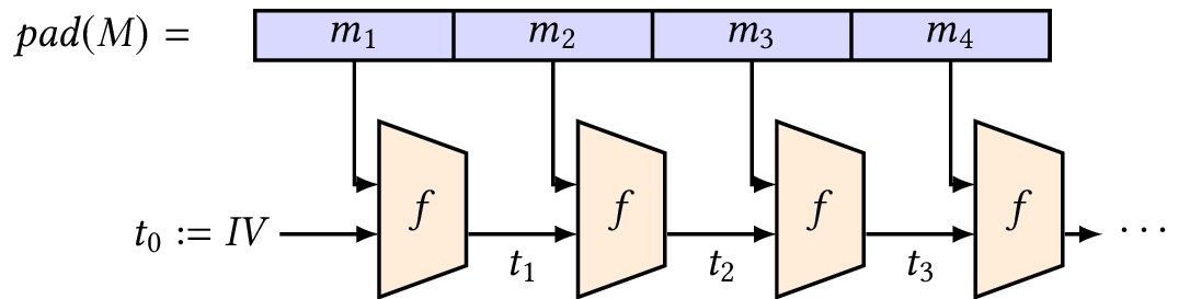
A compression function takes two inputs of some size and produces one output of the size of one of the inputs. Put simply, it takes some data and returns less data. While there are different ways of building a compression function, SHA-2, for example, uses the Davies–Meyer construction (see Figure 1), which relies on a block cipher.
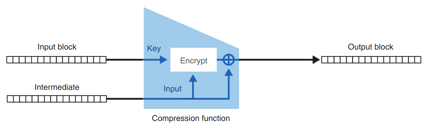
First, it applies a padding to the input we want to hash, then cuts the input into blocks that can fit into the compression function. Cutting the padded input into chunks of the same block size allows us to fit these in the first argument of the compression function. For example, SHA-256 has a block size of \(512\) bits.
Second, it iteratively applies the compression function to the message blocks, using the previous output of the compression function as second argument to the compression function. The final output is the digest.
SHA-3 and the sponge construction
Both the MD5 and SHA-1 hash functions were broken somewhat recently. These two functions made use of the same Merkle–Damgård construction described in the previous section. Because of this, and the fact that SHA-2 is vulnerable to length-extension attacks, NIST decided in 2007 to organize an open competition for a new standard: SHA-3.
In 2007, 64 different candidates from different international research teams entered the SHA-3 contest. Five years later, Keccak, one of the submissions, was nominated as the winner and took the name SHA-3. In 2015, SHA-3 was standardized in the NIST publication FIPS 202.2
SHA-3 is built with a sponge construction, a different construction from Merkle–Damgård that was invented as part of the SHA-3 competition. This is a relatively new way to construct hash functions, since it is built on top of a permutation instead of a compression function. Instead of using a block cipher to mix message bits with the internal state, sponge functions just do an XOR operation. Sponge functions are not only simpler than Merkle–Damgård functions, they’re also more versatile. You will find them used as hash functions and also as deterministic random bit generators, stream ciphers, pseudorandom functions, and authenticated ciphers.
To use a permutation in our sponge construction, we also need to define an arbitrary division of the input and the output into a rate \(r\) and a capacity \(c\). Where we set the limit between the rate and the capacity is arbitrary. Different versions of SHA-3 use different parameters. We informally point out that the capacity is to be treated like a secret, and the larger it is, the more secure the sponge construction.
A sponge function works as follows:
-
It XORs the first message block \(m_1\) to a predefined initial value of the internal state (for example, the all-zero string). Message blocks are all the same size and smaller than the internal state.
-
A permutation \(f\) transforms the internal state to another value of the same size.
-
It XORs block \(m_2\) and applies \(f\) again, and then repeats this for the message blocks \(m_3\), \(m_4\), and so on. This is called the absorbing phase.
-
After injecting all the message blocks, it applies \(f\) again and extracts a block of bits from the state to form the hash. (If you need a longer hash, apply \(p\) again and extract a block.) This is called the squeezing phase.
Because it is a sponge construction, ingesting the input is naturally called absorbing and creating the digest is called squeezing. The sponge is specified with a \(1600\)-bit permutation using different values for \(r\) and \(c\), depending on the security advertised by the different versions of SHA-3.
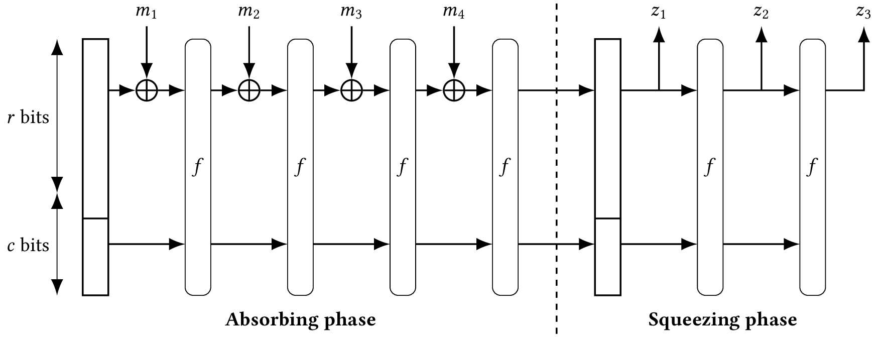
The random-oracle model (optional)
Hash functions are usually designed so that their digests are unpredictable and random. This is useful because one cannot always prove a protocol to be secure, thanks to one of the security properties of a hash function we talked about (like collision resistance, for example). Many protocols are instead proven in the random-oracle model, where a fictional and ideal participant called a random oracle is used. In this type of protocol, one can send any inputs as requests to that random oracle, which is said to return completely random outputs in response, and like a hash function, giving it the same input twice returns the same output twice.
Proofs in this model are sometimes controversial as we don’t know for sure if we can replace these random oracles with real hash functions (in practice). Yet, many legitimate protocols are proven secure using this method, where hash functions are seen as more ideal than they probably are.
Attacks on hash functions
As said before, there’s always ought to be a hash collision for every hash function due to the pigeonhole principle. A simple but inefficient attack based on this is to generate enough hashes so that the digests will repeat at some point. More concretely, if a hash function \(H\) outputs an \(n\)-bit digest, then after hashing \(2^n + 1\) distinct inputs, there must be a collision.
Birthday attacks
The birthday attack gets its name from the birthday paradox: that in a group of \(23\) people, the probability of two people sharing a birthday exceeds \(50%\).
Let \(H\) be a hash function with \(N = 2^n\) possible outputs. The birthday paradox implies that we can find a collision with only \(O(\sqrt{N})\) elements with probability greater than \(\frac{1}{2}\). We can come up with the following algorithm that does the birthday attack:
-
Choose \(k\) uniformly random messages \(m_1, \dots, m_k\).
-
Compute \(t_i \gets H(m_i)\) for every \(i\).
-
Search for \(i\) and \(j\) such that \(m_i \ne m_j\) and \(H(m_i) = H(m_j)\).
This algorithm would end up requiring \(\sqrt{N} = 2^{n/2}\) hash evaluations and \(n\sqrt{N} = n 2^{n/2}\) memory, which makes it no (asymptotically) better than a naïve brute force attack. However, it is possible to find collisions with less memory using Floyd’s cycle-finding algorithm.
The way this works is that we have two “runners,” aptly named the tortoise and the hare, run on a long circular track (which would be our sequence). Like in the story, the hare runs twice as fast as the tortoise. They start off at the same position and when the hare overtakes the tortoise, we know that the hare has cycled around at least once.
-
Start at an arbitrary \(x_0 = y_0\).
-
Compute \(x_i \gets H(x_{i-1})\) (tortoise), \(y_i \gets H(H(y_{i-1}))\) (hare),
-
If \(x_i = y_i\), then \(x_i\) and \(H(y_{i-1})\) are a hash collision.
Here, the hash function serves as a sort of a pseudorandom generator to generate a pseudorandom sequence, which if it behaves “random enough” it guarantees us that there is a cycle of length \(\sqrt{N}\). Floyd’s algorithm runs in \(O(\sqrt{N})\) time (so still exponential in \(n\)), but now it only consumes \(O(1)\) memory, which makes it a massive improvement.
Dictionary attacks
Simply put, a dictionary attack is a form of brute force, but it only
deals with a limited set of possible inputs. This includes words in a
dictionary or previously used passwords acquired from a data breach
(such as the rockyou passwords list).
Since a frequent application of cryptographic hash functions is to store passwords securely, password-cracking software such as Hashcat and John the Ripper typically use dictionary attacks, relying on the fact that people mostly use weak and easy-to-guess passwords.
A speed-up of dictionary attack is through a time–memory trade-off technique, where the hashes of dictionary words are precomputed and storing these in a database using the hash as the key. Most websites that “crack” hashes are simply using precomputed tables, while software such as RainbowCrack uses rainbow tables, which reduce storage requirements at the cost of slightly longer lookup times.
References
-
Aumasson, Jean-Philippe. 2017. Serious Cryptography: A Practical Introduction to Modern Encryption. No Starch Press.
-
Wong, David. 2021. Real-World Cryptography. Manning Publications.
If you want to drill \(n\) holes in \(m\) pigeons where \(n > m\), there will be at least one pigeon with more than one hole.
Message authentication codes
Relevant readings: Katz and Lindell 4.1–4.4, 5.1–5.3, 6.3 (Katz and Lindell 2021), Wong ch. 3, 4.4–4.6 (Wong 2021)
A naïve approach to message integrity
As we have seen from previous lectures, some encryption schemes are malleable, such as a block cipher in CBC mode. As a consequence, an attacker can intercept a message and send a modified message, and the recipient won’t even know the message has been tampered.
A straightforward solution is to include the hash along with the message, thus we now have \(m \mathrel{\hspace{1pt}||\hspace{1pt}}H(m)\). This way, the recipient can use the hash to verify the message. Sounds good, right?
Not so fast. Since it is trivial to recover the hash and the message, an attacker can modify the message and update the hash accordingly, so the attacker then sends \(m^\prime \mathrel{\hspace{1pt}||\hspace{1pt}}H(m^\prime)\). Because both the message and the hash are tampered, the recipient still won’t even know the message has been tampered as the hash agrees with the message!
As anyone including the attacker knows the hash function used to hash the message, a step towards the right direction is to introduce some sort of a key so that nobody but the communicating parties can authenticate and verify their messages.
Message authentication codes
A message authentication code (or MAC) protects a message’s integrity by computing a value \(t \mathrel{\hspace{1pt}\leftarrow\hspace{1pt}}\Mac{k}{m}\) called the tag of the message \(m\). Intuitively, MACs are just hash functions with secret keys.
When one party wants to send a message \(m\) to the other, she computes a tag \(t\) based on the message and the shared key, and sends the message \(m\) along with \(t\) to the other party. The tag is computed using a tag-generation algorithm Mac. Upon receiving \((m,t)\), the second party verifies whether \(t\) is a valid tag on the message \(m\) (with respect to the shared key) or not.
A message authentication code consists of three probabilistic polynomial-time algorithms \((\textsf{Gen}{}, \textsf{Mac}{}, \textsf{Ver}{})\) such that:
-
The key-generation algorithm Gen takes as input the security parameter \(\texttt{1}^n\) and outputs a key \(k\) with \(\Len{k} \ge n\).
-
The tag-generation algorithm Mac takes as a key \(k\) and a message \(m \in \Set{\texttt{0}, \texttt{1}}^*\) and outputs a tag \(t\). Since this algorithm may be randomized, we write this as \(t \mathrel{\hspace{1pt}\leftarrow\hspace{1pt}}\Mac{k}{m}\).
-
The deterministic verification algorithm Ver takes as input a key \(k\), a message \(m\), and a tag \(t\). It outputs a bit \(b\), with \(b = \texttt{1}\) meaning valid and \(b = \texttt{0}\) meaning invalid. We write this as \(b :=\Ver{k}{m, t}\).
It is required that for every \(n\), every key \(k\) output by \(\Gen{\texttt{1}^n}\), and every \(m \in \Set{\texttt{0}, \texttt{1}}^*\), it holds that \(\Ver{k}{m, \Mac{k}{m}} = \texttt{1}\).
Verifying authentication tags
For deterministic MACs (i.e., where Mac is a deterministic algorithm), the canonical way to perform verification is simply to re-compute the tag and check for equality. In other words, \(\Ver{k}{m, t}\) works as follows:
-
Compute \(t^\prime :=\Mac{k}{m}\).
-
Output
1if \(t^\prime = t\) (the tag is valid), otherwise output0.
When verifying an authentication tag, the comparison between the received authentication tag and the one you compute must be done in constant time. This means the comparison should always take the same time, assuming the received one is of the correct size. If the time it takes to compare the two authentication tags is not constant time, it is probably because it returns the moment the two tags differ. This usually gives enough information to enable attacks that can recreate byte by byte a valid authentication tag by measuring how long it takes for the verification to finish.
Security of MACs
The general security goal of a MAC is to prevent authentication tag forgery on a new message.
A message authentication code is considered secure if it is existentially unforgeable, meaning no efficient adversary should be able to generate a valid tag on any “new” message that was not previously sent (and authenticated) by one of the communicating parties.
This notion has an associated game, called the EUF-CMA game, defined for a MAC \(\Pi = (\textsf{Gen}{}, \textsf{Mac}{}, \textsf{Ver}{})\) as follows:
-
A key \(k\) is generated by running \(\Gen{\texttt{1}^n}\).
-
The adversary \(\mathcal{A}\) is given input \(\texttt{1}^n\) and oracle access to \(\Mac{k}{\cdot}\). The adversary eventually outputs \((m, t)\). Let \(\mathcal{Q}\) denote the set of all queries that \(\mathcal{A}\) submitted to its oracle.
-
\(\mathcal{A}\) wins if and only if \(\Ver{k}{m, t} = \texttt{1}\) and \(m \notin \mathcal{Q}\) (i.e., \(\mathcal A\) never queried \(m\)).
Thus a MAC is secure if no efficient adversary can win the game with non-negligible probability.
A message authentication code \(\Pi = (\textsf{Gen}{}, \textsf{Mac}{}, \textsf{Ver}{})\) is existentially unforgeable under an adaptive chosen-message attack, or simply secure, if for all PPT adversaries \(\mathcal{A}\) there is a negligible function \(\mu\) such that: $$\Pr[\text{$\mathcal{A}$ wins the EUF-CMA game}] \le \mu(n).$$
“Strongly secure” MACs
As defined, a secure MAC ensures that an adversary cannot generate a valid tag on a message that was never previously authenticated. But it does not rule out the possibility that an attacker might be able to generate a new, valid tag on a previously authenticated message.
In standard applications of MACs, this type of adversarial behavior is not a concern. Nevertheless, in some settings it is useful to consider a stronger definition of security for MACs where such behavior is ruled out.
Fix a MAC \(\Pi = (\textsf{Gen}, \textsf{Mac}, \textsf{Ver})\), a security parameter \(n\), and a PPT adversary \(\mathcal{A}\). We define the SUF-CMA game as follows:
-
A key \(k\) is generated by running \(\Gen{\texttt{1}^n}\).
-
The adversary \(\mathcal{A}\) is given input \(\texttt{1}^n\) and oracle access to \(\Mac{k}{\cdot}\). The adversary eventually outputs \((m, t)\).
-
\(\mathcal{A}\) wins if and only if \(\Ver{k}{m, t} = \texttt{1}\) and \((m,t)\) was not among the signed pairs.
We then say that \(\Pi\) is strongly secure if the probability of \(\mathcal A\) winning the SUF-CMA game is negligible in \(n\).
In this scenario, the adversary can query the target message but not return one of the responses. This stronger definition ensures that the adversary cannot “maul” the authentication tag.
MACs in practice
CBC-MAC
CBC-MAC is based on a block cipher in CBC mode. Unlike CBC-mode encryption, its starting value is not random (hence it cannot be considered as an IV), and the output is only a single block (representing the tag).
-
Generate key \(k \mathrel{\hspace{1pt}\leftarrow\hspace{1pt}}\Set{\texttt{0}, \texttt{1}}^n\).
-
For input \(m = m_1\cdots m_\ell\), compute \(\Mac{k}{m}\) as follows:
-
Set \(t_0 :=\texttt{0}^n\) (fixed, non-random value).
-
For \(i :=1, \dots, \ell\), set \(t_i :=F_k (t_{i-1} \oplus m_i)\).
-
Output last block \(t_\ell\).
-
-
\(\Ver{k}{m, t}\) returns
1if \(\Mac{k}{m} = t\),0otherwise.
CBC-MAC is secure as long as \(F\) is a secure pseudorandom function (in practice, \(F\) should be some Enc from a well-known block cipher).
Length extension attacks
It’s also possible to construct a MAC from hash functions; however, care must be taken to ensure that the underlying hash function is not vulnerable to a length extension attack. Here’s an example of how not to construct a MAC from a hash function.
Consider a candidate MAC construction, where Mac is defined as: $$\Mac{k}{m} :=H(k \mathrel{\hspace{1pt}||\hspace{1pt}}m).$$ If \(H\) was derived from a Merkle–Damgård construction (like MD5, SHA-1, and SHA-2), we can then carry out a length extension attack on \(H\) in order to forge a valid MAC for \(m\) appended with additional data.1
First, let’s recall how a Merkle–Damgård hash works. Starting from \(t_0\), we apply the compression function \(h\) to each plaintext block and the previous \(t\)-value, thus the final iteration of \(h\) will output the digest of the whole message. Notice that the final output of the hash function is equivalent to an intermediate state of a hash function for a longer message, specifically, for \(m \mathrel{\hspace{1pt}||\hspace{1pt}}\text{padding}(m) \mathrel{\hspace{1pt}||\hspace{1pt}}\cdots\).
For this attack, suppose we have the MAC computed as \(H(k \mathrel{\hspace{1pt}||\hspace{1pt}}m)\) where \(m\) is the message and \(k\) is the secret key. We can then forge a valid MAC by computing the MAC for the extended message \(k \mathrel{\hspace{1pt}||\hspace{1pt}}m \mathrel{\hspace{1pt}||\hspace{1pt}}\text{padding}(k \mathrel{\hspace{1pt}||\hspace{1pt}}m) \mathrel{\hspace{1pt}||\hspace{1pt}}m^\prime\). Since we already know what \(H(k \mathrel{\hspace{1pt}||\hspace{1pt}}m)\) is, we can essentially use this to “restart” the hash function from where it ended when it originally hashed \(k \mathrel{\hspace{1pt}||\hspace{1pt}}m\) by overriding its internal state.
Afterwards, hashing the additional message \(m^\prime\) from this new state is essentially equivalent to hashing \((k \mathrel{\hspace{1pt}||\hspace{1pt}}m \mathrel{\hspace{1pt}||\hspace{1pt}}\text{padding}(k \mathrel{\hspace{1pt}||\hspace{1pt}}m) \mathrel{\hspace{1pt}||\hspace{1pt}}m^\prime \mathrel{\hspace{1pt}||\hspace{1pt}}\text{padding}(m^\prime))\) from the “original” state. The only stipulation though is we need to know how long \(k\) is to compute the padding correctly, but that can be easily determined using brute force.
HMAC
HMAC, like its name indicates, is a way to use hash functions with a key. Using a hash function to build MACs is a popular concept as hash functions have widely available implementations, are fast in software, and also benefit from hardware support on most systems.
For this construction, we define Mac as: $$\Mac{k}{m} :=H \left((k \oplus \textit{opad}) \mathrel{\hspace{1pt}||\hspace{1pt}}H\left( (k \oplus \textit{ipad}) \mathrel{\hspace{1pt}||\hspace{1pt}}m\right) \right),$$ where ipad and opad are padding constants defined as \(\textit{ipad} = \texttt{0x36363636}\dots\) and \(\textit{opad} = \texttt{0x5c5c5c5c}\dots\).
HMAC was constructed this way in order to facilitate proofs. In several papers, HMAC is proven to be secure against forgeries as long as the hash function underneath holds some good properties, which all cryptographically secure hash functions should. Due to this, we can use HMAC in combination with a large number of hash functions. Today, HMAC is mostly used with SHA-2.
Chosen-ciphertext attacks
The strongest security notion in the context of encryption is security against chosen-ciphertext attacks. To recall, a chosen-ciphertext attack is where the adversary can decrypt a ciphertext of its choice.
More formally, the adversary is assumed to have access to the decryption oracle \(\Dec{k}{\cdot}\), in addition to the encryption oracle \(\Enc{k}{\cdot}\).
There are two variants of chosen-ciphertext attacks:
-
Non-adaptive chosen-ciphertext attack (CCA1)
The adversary cannot make further calls to the decryption oracle.
-
Adaptive chosen-ciphertext attack (CCA2)
The adversary continues to have access to encryption and decryption oracles.
A non-adaptive chosen-ciphertext attack is also lunchtime attack2 because it works similarly when an attacker has access to a computer (that can decrypt messages) while its owner has gone out for lunch.
CCA-security
Now we consider the IND-CCA game defined for a private-key encryption scheme \(\Pi = (\textsf{Gen}, \textsf{Enc}, \textsf{Dec})\), a security parameter \(n\), and a PPT adversary \(\mathcal{A}\):
-
A key \(k\) is generated by running \(\Gen{\texttt{1}^n}\).
-
The adversary \(\mathcal{A}\) is given input \(\texttt{1}^n\) and oracle access to \(\Enc{k}{\cdot}\) and \(\Dec{k}{\cdot}\), and outputs a pair of message \(m_{\texttt{0}}\) and \(m_{\texttt{1}}\) of the same length.
-
A uniform bit \(b \in \Set{\texttt{0}, \texttt{1}}\) is chosen, and then a challenge ciphertext \(c \mathrel{\hspace{1pt}\leftarrow\hspace{1pt}}\Enc{k}{m_b}\) is computed and given to \(\mathcal{A}\).
-
\(\mathcal{A}\) continues to have oracle access to \(\Enc{k}{\cdot}\) and \(\Dec{k}{\cdot}\), but is not allowed to query the latter on the challenge ciphertext itself. \(\mathcal{A}\) outputs a bit \(b^\prime\).
-
\(\mathcal{A}\) wins if \(b^\prime = b\).
A private-key encryption scheme \(\Pi = (\textsf{Gen}, \textsf{Enc}, \textsf{Dec})\) has indistinguishable encryptions under a chosen-ciphertext attack, or CCA-secure for short, if for all PPT adversaries \(\mathcal{A}\) there is a negligible function \(\mu\) such that for all \(n\), $$\Pr\left[\text{$\mathcal{A}$ wins the IND-CCA game}\right] \le \tfrac{1}{2} + \mu(n).$$ The probability above is taken over the randomness used by \(\mathcal{A}\) and the randomness used in the game.
Authenticated encryption
Until now, we have considered how to obtain secrecy (using encryption) and integrity (using message authentication codes) separately. We have also witnessed that, on their own, proper encryption is “hard” and proper authentication is “harder” to get right without screwing up. For this reason, a lot of research has emerged seeking to standardize all-in-one constructions that simplify the use of encryption for developers.
The aim of authenticated encryption is to achieve both goals simultaneously. It is best practice to always ensure secrecy and integrity by default in the private-key setting. Indeed, in many applications where secrecy is required it turns out that integrity is essential also. Moreover, a lack of integrity can sometimes lead to a breach of secrecy.
A private-key encryption scheme is an authenticated encryption (AE) scheme if it is CCA-secure and unforgeable.
Let \(\Pi_E = (\textsf{Enc}{}, \textsf{Dec}{})\) be a CPA-secure encryption scheme and let \(\Pi_M = (\textsf{Mac}{}, \textsf{Ver}{})\) denote a strongly secure MAC, where key generation in both schemes simply involves choosing a uniform \(n\)-bit key.
-
Encrypt-and-MAC
Encryption and authentication are done independently. Given a message \(m\), the sender transmits the ciphertext \((c,t)\) where: $$c \mathrel{\hspace{1pt}\leftarrow\hspace{1pt}}\Enc{k_E}{m} \text{ and } t \mathrel{\hspace{1pt}\leftarrow\hspace{1pt}}\Mac{k_M}{m}.$$
-
MAC-then-encrypt
A tag \(t\) is first computed, then the message and tag are encrypted together. Given a message \(m\), the sender transmits the ciphertext \(c\) computed as: $$t \mathrel{\hspace{1pt}\leftarrow\hspace{1pt}}\Mac{k_M}{m} \text{ and } c \mathrel{\hspace{1pt}\leftarrow\hspace{1pt}}\Enc{k_E}{m \mathrel{\hspace{1pt}||\hspace{1pt}}t}.$$
-
Encrypt-then-MAC
The message \(m\) is first encrypted and then a tag is computed over the result. Given a message \(m\), the sender transmits the ciphertext \((c,t)\) where: $$c \mathrel{\hspace{1pt}\leftarrow\hspace{1pt}}\Enc{k_E}{m} \text{ and } t \mathrel{\hspace{1pt}\leftarrow\hspace{1pt}}\Mac{k_M}{c}.$$
Encrypt-and-MAC
In theory, this is the least secure AE construction. Because the goal of using MACs is simply to make tags unforgeable, and because tags aren’t necessarily random looking, the tag \(t\) of a plaintext \(m\) could still leak information even though the MAC is considered secure!
In particular, if a deterministic MAC like CBC-MAC is used, then the tag computed on a message (for some fixed key \(k_M\)) is the same every time. This allows an eavesdropper to identify when the same message is sent twice, something that is not possible for a CPA-secure scheme. Many MACs used in practice are deterministic, so this represents a real concern.
In practice, it has proven good enough for use with SSH, provided that strong MAC algorithms like HMAC-SHA-256 are used.
MAC-then-encrypt
The recipient must decrypt \(c\) before they can determine whether they are receiving corrupted packets, which could expose potentially corrupted plaintexts to the receiver.
For example, consider CBC-mode encryption with padding, where it works by first padding the plaintext (which in our case will be \(m \mathrel{\hspace{1pt}||\hspace{1pt}}t\)) in a specific way so the result is a multiple of the block length, and then encrypting the result using CBC mode. During decryption, if an error in the padding is detected after performing the CBC-mode decryption, then a “bad padding” error is returned. With regard to the MAC-then-encrypt approach, this means there are now two sources of potential decryption failure: the padding may be incorrect, or the tag may not verify.
Nevertheless, it is more secure than encrypt-and-MAC because it hides the plaintext’s authentication tag, thus preventing the tag from leaking information on the plaintext. MAC-then-encrypt has been used in the TLS protocol for years, but TLS 1.3 (the lastest version) replaced MAC-then-encrypt with authenticated ciphers.
Encrypt-then-MAC
This is the most sound approach of the three. One advantage with this method is that the receiver only needs to compute a MAC in order to detect corrupt messages, meaning that there is no need to decrypt a corrupt ciphertext. Another advantage is that attackers can’t send pairs \((c, t)\) to the receiver to decrypt unless they have broken the MAC, which makes it harder for attackers to transmit malicious data to the recipient. This combination of features makes encrypt-then-MAC stronger than the encrypt-and-MAC and MAC-then-encrypt approaches. This is one reason why the widely used IPSec secure communications protocol suite uses it to protect packets (for example, within VPN tunnels).
The cryptographic doom principle
Moxie Marlinspike, creator of the Signal messaging app, proposed a rule of thumb called the “cryptographic doom principle” to determine which among the AE constructions are sound:
When it comes to designing secure protocols, I have a principle that goes like this: if you have to perform any cryptographic operation before verifying the MAC on a message you’ve received, it will somehow inevitably lead to doom.3
Authenticated encryption with associated data
In practice, the more correct answer would be to not bother about how to combine an encryption scheme and a MAC on your own, and just use a pre-defined authentication mode.
The most current way of encrypting data is to use an all-in-one construction called authenticated encryption with associated data (AEAD). The construction is extremely close to what AES-CBC-HMAC provides as it also offers confidentiality of your plaintexts while detecting any modifications that could have occurred on the ciphertexts. What’s more, it provides a way to authenticate associated data.
The associated data argument is optional and can be empty or it can also contain metadata that is relevant to the encryption and decryption of the plaintext. This data will not be encrypted and is either implied or transmitted along with the ciphertext. In addition, the ciphertext’s size is larger than the plaintext because it now contains an additional authentication tag (usually appended to the end of the ciphertext).
To decrypt the ciphertext, we are required to use the same implied or transmitted associated data. The result is either an error, indicating that the ciphertext was modified in transit, or the original plaintext.
Nowadays, the most popular AEAD ciphers are AES-GCM (Galois/Counter mode) and ChaCha20-Poly1305. AES-GCM combines AES in CTR mode with a MAC that works over finite fields (hence the name). ChaCha20-Poly1305 combines the ChaCha20 stream cipher and the Poly1305 MAC algorithm, designed for fast performance in software. For this reason, it is often preferred over AES-GCM for mobile and embedded systems that run ARM-based processors, which cannot take advantage of native x86 instructions dedicated for AES and finite fields.
References
-
Katz, Jonathan, and Yehuda Lindell. 2021. Introduction to Modern Cryptography. 3rd ed. CRC Press.
-
Wong, David. 2021. Real-World Cryptography. Manning Publications.
It’s also worth mentioning that SHA-3 (and other hash functions derived from a sponge construction) is secure against length extension attacks, and so this particular MAC construction is considered secure in those cases.
Hence, https://lunchtimeattack.wtf.
Public-key encryption
Relevant readings: Katz and Lindell 9.3, 11.3–11.4, 12.1, 12.4
Discrete logarithms, again
We recall in this section some facts about cyclic groups from Lecture 4.
Let \(G\) be a (multiplicative) group. Then we define “group exponentiation” as the result of multiplying an element \(x \in G\) with itself \(k\) times: $$x^k = \underbrace{x \cdot x \cdots x}_{\text{$k$ times}}.$$ If \(k = 0\), then \(x^0 = e\), the identity element of \(G\).
A finite group \(G\) is cyclic if there is an element \(g \in G\) such that for all \(x \in G\) there is an integer \(k\) with \(x = g^k\); we call such \(g\) a generator of \(G\). For arbitrary \(a \in G\), the set of all powers of \(a\) forms a cyclic subgroup of \(G\), called the subgroup generated by \(a\), denoted by \(\gen{a}\): $$\gen{a} = \Set{a^0, a^1, \ldots}.$$ If \(g\) is a generator of \(G\), then \(\gen{g} = G\).
Suppose \(G\) is a finite cyclic group of order \(n\), and let \(g\) be a generator of \(G\) and \(h \in G\) be an arbitrary element. The discrete logarithm of \(h\) with respect to \(g\) is the unique integer \(x \in \ZZ_n\) such that \(g^x = h\). Group exponentiation and discrete logarithms are inverses of each other.
Intractable problems involving cyclic groups
We recall several computational problems that can be defined for any class of cyclic groups.
The discrete logarithm problem
The discrete logarithm problem (DLP) in a cyclic group \(G\) with generator \(g\) is to compute \(\log_g h\) for an element \(h \in G\) (i.e., find the unique integer \(x \in \ZZ_n\) for which \(g^x = h\) holds).
The Diffie–Hellman problems
Related (but not equivalent) to the DLP are the Diffie–Hellman problems. There are two important variants: the computational Diffie–Hellman (CDH) problem and the decisional Diffie–Hellman (DDH) problem.
The CDH problem for a cyclic group \(G\) is to compute \(g^{ab}\), given the generator \(g\) and elements \(g^a, g^b\). The CDH assumption is that it is hard to solve the CDH problem, i.e., there’s only a negligible probability of doing so. There is a (polynomial-time) reduction from CDH to DLP, which works as follows:
-
Given \(g^b\), compute \(b\) using an algorithm for DLP.
-
Then compute \(\left(g^a \right)^b = g^{ab}\).
Thus CDH is no harder than DLP, i.e., \(\textsf{CDH} \le_p \textsf{DLP}\).1
The DDH problem for a cyclic group \(G\) is to distinguish \(g^{ab}\) from an element \(g^c\) where \(c \in \ZZ_n\) is chosen uniformly at random. The DDH assumption states that it is hard to do so. There is a (polynomial-time) reduction from DDH to CDH, which works as follows:
-
Given \(g\), \(g^a\), and \(g^b\), compute \(g^{ab}\) using an algorithm for CDH.
-
Then check whether \(g^{ab} = g^c\).
Thus DDH is no harder than CDH, i.e., \(\textsf{DDH} \le_p \textsf{CDH}\).
Key exchange and Diffie–Hellman
The key exchange problem
Since private-key cryptography uses the same secret key for encryption and decryption, it begs the question that we haven’t addressed yet:
How can the parties share a secret key in the first place?
The key cannot just be sent over the insecure communication channel because an eavesdropping adversary would then be able to observe the key, thus it would no longer be secret.
One way to address this issue is to establish a key-distribution center (KDC). But such an approach to the key-distribution problem still require, at some point, a private and authenticated channel that can be used to share keys, which is impractical for open systems like the Internet.
The Diffie–Hellman protocol
In 1976, Whitfield Diffie and Martin Hellman published a paper titled “New Directions in Cryptography.” They observed that there are particular actions that are easy to do but difficult to undo, like it’s easy to shatter a glass vase but extremely difficult to put it back together. These actions can be used to derive interactive protocols for secure key exchange by having the parties perform operations that an eavesdropper cannot reverse.
This insight lead to one of the first steps toward moving cryptography out of the private domain and into the public one. To quote (Diffie and Hellman 1976):
We stand today on the brink of a revolution in cryptography. The development of cheap digital hardware has freed it from the design limitations of mechanical computing and brought the cost of high grade cryptographic devices down to where they can be used in such commercial applications as remote cash dispensers and computer terminals. In turn, such applications create a need for new types of cryptographic systems which minimize the necessity of secure key distribution channels …. At the same time, theoretical developments in information theory and computer science show promise of providing provably secure cryptosystems, changing this ancient art into a science.
We now describe the key exchange protocol that appeared in the original paper by Diffie and Hellman:
-
Alice and Bob agree upon a cyclic group \(G\) of order \(q\) (where \(q\) is \(n\) bits long) and a generator \(g \in G\).
-
Alice chooses \(a \getsrandom \ZZ_q\) uniformly at random and sends \(h_A \gets g^a\) to Bob.
-
Bob receives \(h_A\), then chooses \(b \getsrandom \ZZ_q\) uniformly at random and sends \(h_B \gets g^b\) to Alice.
-
Alice receives \(h_B\), and computes the shared key \(k_A \gets h_B^a = (g^b)^a = g^{ab}\).
-
Bob computes the shared key \(k_B \gets h_A^b = (g^a)^b = g^{ab}\).
Here, the shared key is a group element, not a bit string.
At the time, they did not provide a proof of security of their protocol mainly because the framework for formulating precise security notions, like what we have today, were not yet in place. Rather, the minimal requirement for security here is that the discrete logarithm problem must be hard relative to the underlying group \(G\). This is necessary but not sufficient, as it is possible that there are other ways of computing the key \(k_A = k_B\) without explicitly computing \(a\) or \(b\).
To be considered secure, the shared key \(g^{ab}\) should be indistinguishable from a group element picked uniformly at random for any adversary given \(g\), \(g^a\), and \(g^b\), which is exactly the decisional Diffie–Hellman (DDH) assumption. Thus a proof of security for the Diffie–Hellman protocol follows almost immediately from the DDH assumption.
Diffie–Hellman in practice
Though the Diffie–Hellman protocol in its basic form is not used in practice because it is insecure against man-in-the-middle attacks, it is found at the core of standardized key exchange protocols that are resilient to man-in-the-middle attacks, most notably in the Transport Layer Security (TLS) protocol.
Introducing public-key cryptography
Aside from a key exchange protocol, Diffie and Hellman introduced the notion of public-key cryptography. Instead of having a secret key for both encryption and decryption, we now have a pair of keys: a public key that is widely disseminated, and a private key that is kept secret. For this reason public-key cryptography is sometimes called asymmetric-key cryptography. Having generated these keys, a party can use them to ensure confidentiality for messages it receives using a public-key encryption scheme, or integrity for messages it sends using a digital signature scheme. Table 1 summarizes the cryptographic primitives in both the private-key setting and the public-key setting.
| private-key setting | public-key setting | |
|---|---|---|
| confidentiality | private-key encryption | public-key encryption |
| integrity | message authentication codes | digital signature schemes |
Cryptographic primitives in the private-key and the public-key settings (Katz and Lindell 2021)
Why still study private-key cryptography?
There’s no doubt that public-key cryptography is strictly stronger than private-key cryptography. But the answer to the question is simple: private-key cryptography is much more efficient than public-key cryptography, and should be used in settings where it is appropriate.
For example, we don’t use public-key cryptography to directly encrypt the actual message we want to send, but rather, we use it to encrypt the (symmetric) key used to encrypt the message, which was encrypted using private-key cryptography.2
The public-key encryption syntax
Like what we did in Lecture 1, we formally define a public-key encryption scheme as follows:
A public-key encryption scheme \(\Pi\) is a triple of probabilistic polynomial-time algorithms \((\textsf{Gen}, \textsf{Enc}, \textsf{Dec})\) such that:
-
The key-generation algorithm Gen takes as input the security parameter \(\texttt{1}^n\) and outputs a pair of keys \((\pk, \sk)\), where \(\pk\) is the public key and \(\sk\) is the private key. We assume for convenience that \(\pk\) and \(\sk\) each has length at least \(n\), and that \(n\) can be determined from \(\pk\) and \(\sk\).
The public key \(\pk\) defines a message space \(\mathcal{M}_{\pk}\).
-
The encryption algorithm Enc takes as input a public key \(\pk\) and a message \(m \in \mathcal{M}_{\pk}\), and outputs a ciphertext \(c\). We write this as \(c \getsrandom \Enc{\pk}{m}\).
-
The deterministic decryption algorithm Dec takes as input a private key \(\sk\) and a ciphertext \(c\), and outputs a message \(m\) or \(\bot\) denoting failure. We write this as \(m \gets \Dec{\sk}{c}\).
It is required that, except with negligible probability over the randomness of Gen and Enc, we have \(\Dec{\sk}{\Enc{\pk}{m}} = m\) for any message \(m \in \mathcal{M}_{\pk}\).
Security against chosen-plaintext attacks
We recall the IND-EAV game from Lecture 6, but we now define it for a public-key encryption scheme \(\Pi = (\textsf{Gen}, \textsf{Enc}, \textsf{Dec})\) and an adversary \(\mathcal{A}\) as follows:
-
\(\Gen{\texttt{1}^n}\) is run to obtain keys \((\pk, \sk)\).
-
The adversary \(\mathcal{A}\) is given \(\pk\) and outputs a pair of messages \(m_{\texttt{0}}, m_{\texttt{1}} \in \mathcal{M}_{\pk}\) of equal length.
-
A uniform bit \(b \in \Set{\texttt{0}, \texttt{1}}\) is chosen. Then the ciphertext \(c \getsrandom \Enc{\pk}{m_b}\) is computed and given to \(\mathcal{A}\). We refer to \(c\) as the challenge ciphertext.
-
\(\mathcal{A}\) outputs a bit \(b^\prime\).
-
\(\mathcal{A}\) wins if \(b^\prime = b\).
A public-key encryption scheme \(\Pi = (\textsf{Gen}, \textsf{Enc}, \textsf{Dec})\) has indistinguishable encryptions in the presence of an eavesdropper, or EAV-secure for short, if for all PPT adversaries \(\mathcal{A}\) there is a negligible function \(\mu\) such that for all \(n\), $$\Pr\left[\text{$\mathcal{A}$ wins the IND-EAV game}\right] \le \tfrac{1}{2} + \mu(n).$$ The probability above is taken over the randomness used by \(\mathcal{A}\) and the randomness used in the game.
The main difference between the IND-EAV game presented here and that from Lecture 7 is that here \(\mathcal{A}\) is given the public key \(\pk\). Furthermore, we allow \(\mathcal{A}\) to choose their messages \(m_{\texttt{0}}\) and \(m_{\texttt{1}}\) based on this public key. This is essential when defining security of public-key encryption since it makes sense to assume that the adversary knows the public key of the recipient.
In effect, we’re giving away \(\mathcal{A}\) access to the encryption oracle for free! This makes sense since \(\mathcal{A}\) is assumed to know the algorithm Enc, thus given \(pk\), they can encrypt any message \(m\) by simply computing \(\Enc{\pk}{m}\). As a consequence, EAV-security and CPA-security are equivalent in the public-key setting:
This is unlike in private-key encryption, where there are schemes that are EAV-secure but not CPA-secure.
ElGamal encryption
In 1985, Taher ElGamal observed that the Diffie–Hellman protocol can be adapted to give a public-key encryption scheme, which paved the way to the ElGamal cryptosystem, which we will describe below.
Let \(G\) be a cyclic group and a generator \(g \in G\) such that the DDH assumption holds in \(G\). Then the ElGamal cryptosystem defines a triple of PPT algorithms \((\textsf{Gen}, \textsf{Enc}, \textsf{Dec})\) as follows:
Gen(\(\texttt{1}^n\)):
1: \(x \getsrandom \ZZ_q\)
2: \(h \gets g^x\)
3: \(\pk \gets h\)
4: \(\sk \gets x\)
5: return \((\pk, \sk)\)
Enc(\(\pk\), \(m\)):
1: \(h \gets \pk\)
2: \(y \getsrandom \ZZ_q\)
3: return \((g^y, h^y \cdot m)\)
Dec(\(sk\), \(c\)):
1: \(x \gets \sk\)
2: \((c_1, c_2) \gets c\)
3: \(\hat{m} \gets c_2 / c_1^x\)
4: return \(\hat{m}\)
To see that decryption succeeds, let \((c_1, c_2) = (g^y, h^y \cdot m)\) with \(h = g^x\). Then $$\hat{m} = \frac{c_2}{c_1^x} = \frac{h^y \cdot m}{\left(g^y\right)^x} = \frac{\left(g^x\right)^y \cdot m}{g^{xy}} = \frac{g^{xy} \cdot m}{g^{xy}} = m.$$
Let \(q=83\) and \(p = 2q+1 = 167\), and let \(G\) denote the group of quadratic residues modulo \(p\). Since the order of \(G\) is prime, any element of \(G\) except \(1\) is a generator, thus we take \(g = 2^2 \equiv 4 \pmod{167}\). Suppose Bob chooses the secret key \(37 \in \ZZ_{83}\) and so the public key is $$\pk = 4^{37} \bmod 167 = 76.$$
Suppose Alice encrypts the message \(m = 65 \in G\) (note that \(65 = 30^2 \bmod 167\) and so \(65\) is an element of \(G\)). If \(y = 71\), the ciphertext is $$(4^{71} \bmod 167, 76^{71} \cdot 65 \bmod 167) = (132, 44).$$
To decrypt, Bob first computes \(132^{37} \bmod 167 = 124\), then since \(124^{-1} \bmod 167 = 66\), he recovers \(m = 44 \cdot 66 \bmod 167 = 65\).
References
-
Diffie, Whitfield, and Martin E. Hellman. 1976. "New Directions in Cryptography." IEEE Transactions on Information Theory 22 (6): 644--54. https://doi.org/10.1109/TIT.1976.1055638.
-
Katz, Jonathan, and Yehuda Lindell. 2021. Introduction to Modern Cryptography. 3rd ed. CRC Press.
The direction of the reduction is very important! As a rule of thumb, you always reduce from a problem you don’t know to another problem you already know.
Algorithmic number theory
Relevant readings: CLRS 31.8–31.9, Katz and Lindell 9.2, 10.1–10.2, App. B
Primality testing
Distribution of primes
Recall from Lecture 3 that although there’s no clear pattern about the distribution of prime numbers, one of the great insights about them is that their density among the integers has a precise limit, which is described by the prime number theorem.
The approximation \(n / \ln n\) gives reasonably accurate estimates of \(\pi(n)\) even for small \(n\). For example, it is off by less than \(6%\) at \(n = 10^9\), where \(\pi(n) = 50847534\) and \(n/ \ln n = 48 254942\).
By the prime number theorem, the probability that \(n\) is prime is approximately \(1 / \ln n\), and so we would expect to examine approximately \(\ln n\) integers chosen randomly near \(n\) in order to find a prime that is of the same length as \(n\). For example, we expect that finding a \(1024\)-bit prime would require testing approximately \(\ln 2^{1024} \approx 710\) randomly chosen \(1024\)-bit numbers for primality. Of course, we can cut this figure in half by choosing only odd integers.
Fermat’s pseudoprime test
We now consider a method for primality testing that “almost works” and in fact is good enough for many practical applications.
Recall that Fermat’s little theorem says that for any integer \(a>0\) and prime \(n\), $$a^{n-1} \equiv 1 \pmod{n}. \label{eq:fermat_little}$$
However, if \(n\) is composite and still satisfies the above equation, then we say that \(n\) is a base-\(a\) pseudoprime. Thus, if we can find any \(a\) such that \(n\) does not satisfy the equation, then \(n\) is certainly composite. Surprisingly, the converse almost holds, so that this criterion forms an almost perfect test for primality. We test to see whether \(n\) satisfies equation [eq:fermat_little] for \(a = 2\). If not, we declare \(n\) to be composite by returning “composite.” Otherwise, we return “prime,” guessing that \(n\) is prime, when in fact, all we know is that \(n\) is either prime or a base-\(2\) pseudoprime.
FermatTest(\(n\)):
1: if FastModExp\((a, n-1, n) \ne 1\) // if \(a^{n-1} \not\equiv 1 \pmod{n}\)
2: return “composite” // definitely
3: else
4: return “prime“ // perhaps
This algorithm can make errors, but only of one type. That is, if it says that \(n\) is composite, then it is always correct. If it says that \(n\) is prime, however, then it makes an error only if \(n\) is a base-\(2\) pseudoprime.
How often does this algorithm output the wrong answer? Surprisingly rarely. There are only \(22\) values of \(n\) less than \(10000\) for which it is wrong; the first four such values are \(341\), \(561\), \(645\), and \(1105\). We won’t prove it, but the probability that this algorithm makes an error on a randomly chosen \(m\)-bit number goes to zero as \(m \to \infty\).
The upshot is that if you are merely trying to find a large prime for some application, for all practical purposes you almost never go wrong by choosing large numbers at random until one of them causes FermatTest to return “prime.” But when the numbers being tested for primality are not randomly chosen, we need a better approach for testing primality.
Miller–Rabin primality test
The Miller–Rabin primality test overcomes the problems of the simple Fermat’s pseudoprime test with two modifications:
-
It tries several randomly chosen base values \(a\) instead of just one base value.
-
While computing each modular exponentiation, it looks for a nontrivial square root of \(1\) modulo \(n\), during the final set of squarings. If it finds one, it stops and returns “composite.”
MillerRabin(\(n\), \(t\)):
1: for \(j \gets 1 \ \textbf{to}\ t\)
2: \(a \getsrandom \Set{1, \dots, n-1}\)
3: if Witness(\(a\), \(n\))
4: return “composite” // definitely
5: return “prime” // almost surely
Integer factorization
Suppose we have an integer \(n\) that we wish to factor, that is, to decompose into a product of primes. The primality test of the preceding section may tell us that \(n\) is composite, but it does not tell us the prime factors of \(n\). Factoring a large integer \(n\) seems to be much more difficult than simply determining whether \(n\) is prime or composite. Even with today’s supercomputers and the best algorithms to date, we cannot feasibly factor an arbitrary \(1024\)-bit number.
Trial division
The most straightforward way to factor an integer \(n\) is to try every possible factor; this is called trial division. We try dividing \(n\) by each integer \(2, 3, \dots, \lfloor \sqrt{n} \rfloor\). (We may skip even integers greater than 2.) It is easy to see that \(n\) is prime if and only if none of the trial divisors divides \(n\). Assuming that each trial division takes constant time, the worst-case running time is \(O(\sqrt{n})\), which is exponential in the length of \(n\).
Pollard’s \(\rho\) algorithm
Pollard’s \(\rho\) (“rho”) algorithm can be used to factor an arbitrary integer \(n = pq\); in that sense, it is a general-purpose factoring algorithm. The core idea of the approach is to find distinct values \(x, x^\prime \in \ZZ_n^*\) that are equivalent modulo \(p\) (that is, if \(x \equiv x^\prime \pmod{p}\)); we call such a pair good. Note that for a good pair \(x, x^\prime\) it holds that \(\gcd(x-x^\prime, n ) = p\), since \(x \not\equiv x^\prime \pmod{n}\), so computing the gcd gives a nontrivial factor of \(n\).
The algorithm involves generating a pseudorandom sequence, which is done by a function \(f\). In other words, we will keep applying \(f\) and it will generate numbers that “look and feel” random. (Note that it can never be truly random because this entire sequence can be determined from the choice of \(f\) and the starting value.) Not every function does it but one such function that has this pseudorandom property is \(f(x) \gets (x^2+c) \bmod n\), where \(c\) is usually assumed to be \(1\) in practice.
We define our starting value to be \(x_0 \gets 2\), but any other integer could work. To get the next element \(x_1\) in the sequence, we compute \(x_1 \gets f(x_0)\), and to get the element after that \(x_2\), we compute \(x_2 \gets f(x_1)\). In general, we have the recurrence \(x_{i+1} \gets f(x_i)\).
Suppose \(n = 95\) and \(f(x) \gets (x^2+1) \bmod n\). We show how to derive the pseudorandom sequence in the following table:
| \(x_i\) | \(x_{i+1}\) | \(g \gets \gcd(\abs{x_i - x_{i-1}}, n)\) |
|---|---|---|
| \(2\) | \(5\) | \(\gcd(3, 95) = 1\) |
| \(5\) | \(26\) | \(\gcd(21, 95) = 1\) |
| \(26\) | \(12\) | \(\gcd(14, 95) = 1\) |
| \(12\) | \(50\) | \(\gcd(38, 95) = 19\) |
The last pair of \(x_i, x_{i+1}\) is good since the last value of \(g\) is greater than \(1\), so this must be a nontrivial factor of \(n\). Thus we have found \(19\) as a prime factor of \(95\).
You can see that in many cases this works. But in some cases, it goes into an infinite loop because the function \(f\) gets trapped into a cycle. When that happens, we keep repeating the same set of value pairs \(x_i\) and \(x_{i+1}\) and never stop. For example, if \(n = 55\) and \(f\) is the same as defined previously, the pseudorandom sequence would be: $$2, 5, \textcolor{tomred}{26, 17, 15, 6, 37, 50, 26}, 17, 15, 6, 37, 50, 26, 17, 15, 6, \dots.$$ In this case, we will keep cycling and never find a factor. How do we detect that there is a cycle?
A simple solution is to store all the numbers seen so far \(x_1, \dots, x_n\) in some data structure, and see if \(x_i = x_j\) for some previous \(i < j\). However, doing so would take \(O(n)\) memory, and for very large values of \(n\) (as it usually is in practice) it is infeasible.
A more efficient solution relies on another algorithm to find cycles called Floyd’s algorithm. We have already seen how Floyd’s algorithm works in the context of finding hash collisions, but the idea remains the same:
PollardRho(\(n\)):
1: \(\textit{tortoise} \gets x_0\)
2: \(\textit{hare} \gets x_0\)
3: \(\textit{tortoise} \gets f(\textit{tortoise})\) // tortoise moves one step forward
4: \(\textit{hare} \gets f(f(\textit{hare}))\) // hare moves two steps forward
5: \(g \gets \gcd(\abs{\textit{tortoise} - \textit{hare}}, n)\)
6: if \(1 < g < n\)
7: return \(g\)
8: else if \(g \mathrel{=}n\)
9: return “fail”
The running time of Pollard’s \(\rho\) algorithm turns out to be \(O(\sqrt{p})\) where \(p\) is the smallest divisor that divides \(n\). If \(p\) just so happens to be really small, this algorithm is practically efficient no matter how enormous \(n\) can be. But in the worst case, \(n\) is a product of two equally-sized prime factors, so each of the factors has half the number of bits of \(n\), which means that the running time in terms of \(n\) will be \(O(n^{1/4})\).
Fun fact: The main reason why this algorithm is called the \(\rho\) algorithm is because of the shape that the pseudorandom sequence produces:
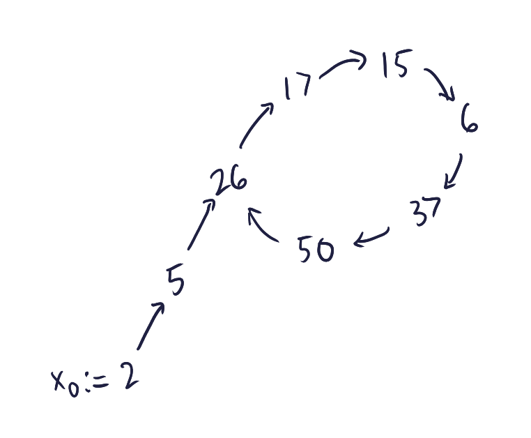
Computing discrete logarithms
Let \(G\) be a cyclic group of known order \(q\). An instance of the discrete logarithm problem in \(G\) specifies a generator \(g \in G\) and an element \(h \in G\); the goal is to find \(x \in \ZZ_q\) such that \(g^x = h\).
A trivial brute-force solution can be done in \(O(q)\) time by iterating through every possible value of \(x\):
NaïveDLog(\(g\), \(h\), \(q\)):
1: for \(x \gets 0 \ \textbf{to}\ q-1\)
2: if \(g^x \mathrel{=}h\)
3: return \(x\)
4: return “fail”
Note that this runs in time exponential to the number of bits of \(q\).
Baby-step giant-step algorithm
A more efficient way to compute discrete logarithms is called the baby-step giant-step algorithm, attributed to Daniel Shanks, which is actually a slight modification of the straightforward solution above. This algorithm is based on a time–memory trade-off, which reduces computing time but comes at the expense of additional memory consumption.
The idea is simple. Given a generator \(g \in G\), we can imagine the powers of \(g\) as forming a cycle $$1 = g^0, g^1, g^2, \dots, g^{q-2}, g^{q-1}, g^q = 1.$$ We know that \(h\) must lie somewhere in this cycle. Computing all the points in this cycle to find \(h\) would take at least time linear in \(q\). Instead, we “mark off” the cycle at intervals of size \(t \gets \lfloor \sqrt{q} \rfloor\). More precisely, we compute and store the \(\lfloor q/t \rfloor + 1 = O(\sqrt{q})\) elements $$g^0, g^t, g^{2t}, \dots, g^{\lfloor q/t \rfloor \cdot t}.$$ These elements are the “giant steps.” Note that the gap between any consecutive “marks” (wrapping around at the end) is at most \(t\). Furthermore, we know that \(h = g^x\) lies in one of these gaps. Thus, if we take “baby steps” and compute the \(t\) elements $$h \cdot g^1, h \cdot g^2, \dots, h \cdot g^t,$$ each of which corresponds to a “shift” of \(h\), we know that one of these values will be equal to one of the marked points. Suppose we find \(h \cdot g^i = g^{k \cdot t}\). We can then easily compute \(\log_g h \gets (k\cdot t - i) \bmod q\).
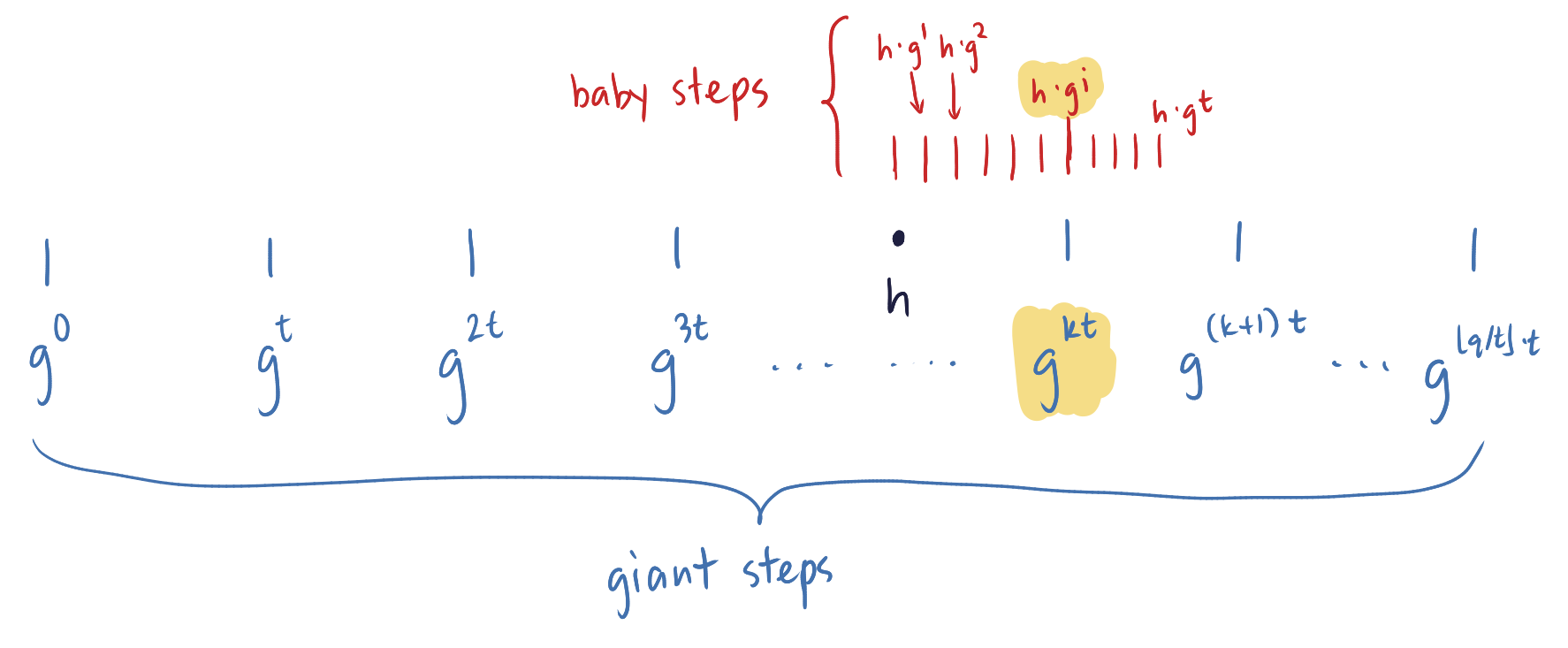
The following pseudocode summarizes this strategy:
BSGS(\(g\), \(h\), \(q\)):
1: \(t \gets \lfloor \sqrt{q} \rfloor\)
2: for \(i \gets 0 \ \textbf{to}\ \lfloor q/t \rfloor\) // giant step
3: \(g_i \gets g^{i \cdot t}\)
4: store the pair \((i, g_i)\) in a lookup table
5: sort the lookup table by the second component // sort by \(g_i\)
6: for \(i \gets 1 \ \textbf{to}\ t\) // baby step
7: \(h_i \gets h \cdot g^i\)
8: if \(h_i \mathrel{=}g_k\) for some \(k\) // use the lookup table to do this
9: return \((k \cdot t - i) \bmod q\)
10: return “fail” // discrete log does not exist
Since \(t = O(\sqrt{q})\), the algorithm runs in \(O(\sqrt{q})\) time, but it also consumes \(O(\sqrt{q})\) space due to the lookup table. Though this seems like a massive improvement over the naïve discrete log algorithm, keep in mind that this still runs in exponential time in the number of bits of \(q\).
References
-
Cormen, Thomas H., Charles E. Leiserson, Ronald L. Rivest, and Clifford Stein. 2009. Introduction to Algorithms. 3rd ed. MIT Press.
-
Katz, Jonathan, and Yehuda Lindell. 2021. Introduction to Modern Cryptography. 3rd ed. CRC Press.
RSA
Relevant readings: Aumasson ch. 10, Katz and Lindell 12.5, Wong 6.3
RSA encryption
Textbook RSA
We first describe the simplest form of RSA called “textbook RSA.” By itself it is insecure, but it serves as a stepping stone for more secure schemes that are actually used in practice.
Let GenRSA be a PPT algorithm that, given \(\texttt{1}^n\), outputs a modulus \(N\) that is the product of two \(n\)-bit primes, along with integers \(e,d\) satisfying \(ed \equiv 1 \pmod{\phi(N)}\). We use an algorithm called GenModulus as a subroutine that outputs a composite modulus \(N\) along with its factorization.
GenRSA(\(\texttt{1}^n\)):
1: \((N, p, q) \getsrandom \text{\CallSpec{GenModulus}{$\texttt{1}^n$}}\)
2: \(\phi(N) \gets (p-1) \cdot (q-1)\)
3: choose \(e\) such that \(\gcd(e, \phi(N)) \mathrel{=}1\)
4: \(d \gets e^{-1} \bmod \phi(N)\)
5: return \(N, e, d\)
We can implement GenModulus in SageMath
using the random_prime function to generate primes:1
def rsa_genmodulus(n):
    p = random_prime(2^n-1, lbound=2^(n-1), proof=False)
    q = random_prime(2^n-1, lbound=2^(n-1), proof=False)
    N = p*q
    return N, p, q
# generate 256-bit RSA modulus
rsa_genmodulus(256)
# generate 512-bit RSA modulus
rsa_genmodulus(512)
As random_prime verifies if the generated prime is actually prime,
this can potentially slow down our rsa_genmodulus function, so we
supply an additional parameter proof=False to random_prime to skip
this verification step.
Suppose \(N, e, d\) are defined as above, and let \(c = m^e \bmod N\) for some \(m \in \ZZ_N^*\). RSA encryption works because someone who has \(d\) can recover \(m\) from \(c\) by computing \(c^d \bmod N\), since: $$c^d = \left(m^e\right)^d = m^{ed} \equiv m \pmod{N}.$$ If \(d\) is not known, then the RSA assumption (from Lecture 5) says that it is difficult to recover \(m\) from \(c\) even if \(N\) and \(e\) are known. In this sense, computing \(m^e \bmod N\) is a trapdoor and \(d\) is the ladder that we use to get out. We define the textbook RSA scheme as follows:
-
Gen: given \(\texttt{1}^n\) run to obtain \(N\), \(e\), and \(d\). The public key is \((N, e)\) and the private key is \((N, d)\).
-
Enc: given a public key \(\pk = (N, e)\) and a message \(m \in \ZZ_N^*\), compute the ciphertext $$c \gets m^e \bmod N.$$
-
Dec: given a private key \(\sk = (N, d)\) and a ciphertext \(c \in \ZZ_N^*\), compute the message $$m \gets c^d \bmod N.$$
Say GenRSA outputs \((N, e, d) = (391, 3, 235)\), so the public key is \((391, 3)\) and the private key is \((391, 235)\).
To encrypt the message \(m = 158 \in \ZZ_{391}^*\) using the public key \((391,3)\), we simply compute \(c \gets 158^3 \bmod 391 = 295\) which is the ciphertext. To decrypt, the receiver computes \(295^{235} \bmod 391 = 158\).
Since Enc is deterministic (notice that we don’t use any randomness for encryption), it is not CPA-secure.
Padded RSA
To make textbook RSA CPA-secure, we need encryption to be nondeterministic (i.e., randomized). One way to do this is to randomly pad the message before encrypting. More concretely, to map a message \(m\) to an element of \(\ZZ_N^\), the sender chooses a uniform bit-string \(r \in \Set{\texttt{0}, \texttt{1}}^\ell\) (for some appropriate \(\ell\)) and sets \(\hat{m} \gets r \mathrel{\hspace{1pt}||\hspace{1pt}}m\); the resulting value can naturally be interpreted as an integer in \(\ZZ_N^\). We can see that this mapping is reversible, as we can simply chop off the extra bits after decryption.
Let GenRSA be as before, and let \(\ell\) be a function with \(\ell(n) < 2n\). We define the padded RSA scheme as follows:
-
Gen: given \(\texttt{1}^n\) run to obtain \(N\), \(e\), and \(d\). The public key is \((N, e)\) and the private key is \((N, d)\).
-
Enc: given a public key \(\pk = (N, e)\) and a message \(m \in \Set{\texttt{0}, \texttt{1}}^{q - \ell(n) - 1}\) (where \(N\) is \(q\) bits long), choose a string \(r \in \Set{\texttt{0}, \texttt{1}}^\ell\) and interpret \(\hat{m} \gets r \mathrel{\hspace{1pt}||\hspace{1pt}}m\) as an element of \(\ZZ_N^*\), then compute the ciphertext $$c \gets \hat{m}^e \bmod N.$$
-
Dec: given a private key \(\sk = (N, d)\) and a ciphertext \(c \in \ZZ_N^*\), compute the message $$\hat{m} \gets c^d \bmod N,$$ and output the \(q - \ell(n) - 1\) least significant bits of \(\hat{m}\).
PKCS#1 v1.5
The PKCS#1 v1.5 standard, published in 1993, defines a variant of padded
RSA. For a public key \(\pk = (N, e)\), let \(k\) denote the length
of \(N\) in bytes. We assume that a message \(m\) to be encrypted
has a length an integer number of bytes ranging from \(1\) to
\(k-11\). Encryption of a \(D\)-byte message \(m\) is computed as
$$(\texttt{0x00} \mathrel{\hspace{1pt}||\hspace{1pt}}\texttt{0x02} \mathrel{\hspace{1pt}||\hspace{1pt}}r \mathrel{\hspace{1pt}||\hspace{1pt}}\texttt{0x00} \mathrel{\hspace{1pt}||\hspace{1pt}}m)^e \bmod N,$$
where \(r\) is a randomly generated \((k-D-3)\)-byte string with
none of its bytes equal to 0x00.
Since a devastating chosen-ciphertext attack due to Bleichenbacher has been demonstrated against PKCS#1 v1.5, newer versions of the standard have been introduced.2
RSA-OAEP and PKCS#1 v2
A bigger problem with textbook RSA is that it is malleable. In this case, given the encryption \(c = m^e \bmod N\) of some unknown message \(m\), it’s easy to generate a related ciphertext \(c^\prime\) that is an encryption of \(2m \bmod N\) by setting: $$c^\prime \gets 2^e \cdot c \bmod N = 2^e \cdot m^e = (2m)^e \bmod N.$$ In fact, if we have two ciphertexts \(c_1 = m_1^e \bmod N\) and \(c_2 = m_2^e \bmod N\), we can derive the ciphertext of \(c_1 \cdot c_2\) by multiplying these two ciphertexts together, like this: $$(c_1 \cdot c_2) \bmod N = (m_1^e \cdot m_2^e) \bmod N = (m_1 \cdot m_2)^e \bmod N.$$ Thus we now have the ciphertext of the message \(m_1 \cdot m_2\).
In order to make RSA ciphertexts nonmalleable, the ciphertext should consist of the message data and some padding. Another way of padding the message is the optimal asymmetric encryption padding (OAEP), commonly referred to as RSA-OAEP, which is standardized as part of the PKCS#1 v2 standard. This scheme involves creating a bit string as large as the modulus by padding the message with extra data and randomness before applying the RSA function. Unlike its predecessor, PKCS#1 v1.5, OAEP is not vulnerable to Bleichenbacher’s attack and is, thus, a strong standard to use for RSA encryption nowadays. Let’s see how OAEP works and prevents the previously discussed attacks.
Like most cryptographic algorithms, OAEP comes with a key-generation algorithm, which takes the security parameter \(\texttt{1}^n\) as input. As with Diffie–Hellman, operations happen in the ring of integers modulo a large number. When we talk about the security of an instantiation of RSA, we usually refer to the size of that large modulus. This is similar to Diffie–Hellman if you remember.
To encrypt, the algorithm first pads the message and mixes it with a random number generated per encryption. The result is then encrypted with RSA. To decrypt the ciphertext, the process is reversed as Figure 1 shows. RSA-OAEP uses this mixing in order to make sure that if a few bits of what is encrypted with RSA leak, no information on the plaintext can be obtained. Indeed, to reverse the OAEP padding, you need to obtain (close to) all the bytes of the OAEP padded plaintext! In addition, Bleichenbacher’s attack should not work anymore because the scheme makes it impossible to obtain well-formed plaintext by modifying a ciphertext.
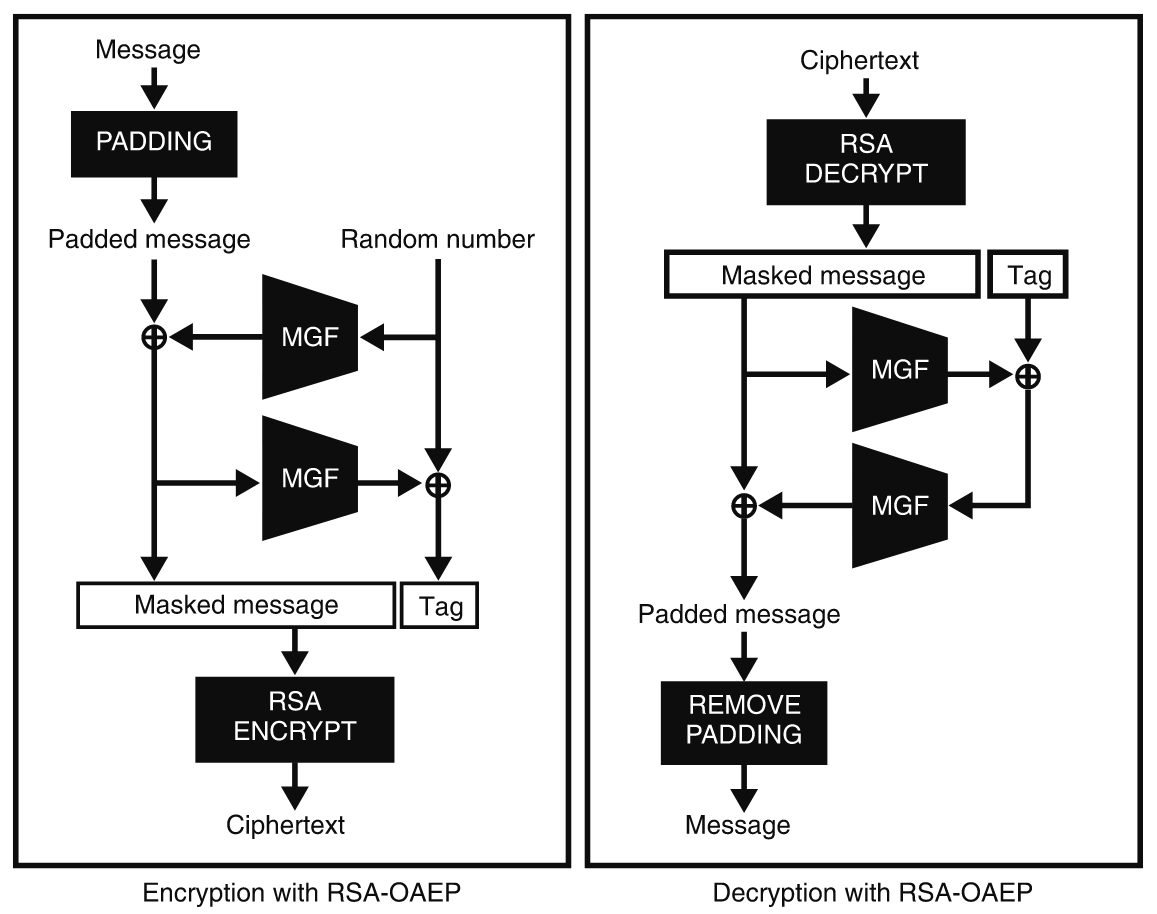
Inside of OAEP, MGF stands for mask generation function. MGFs are built using a hash function that hashes the input repeatedly with a counter (sort of like “a hash function in CTR mode”).
The takeaway here is that always use OAEP whenever you use RSA. Nowadays, most protocols and applications that use RSA either still implement the insecure PKCS#1 v1.5 or OAEP. On the other hand, more and more protocols are moving away from RSA encryption in favor of elliptic curve Diffie–Hellman (ECDH). for both key exchanges and hybrid encryption. This is understandable as ECDH provides shorter public keys and benefits, in general, from much better standards and much safer implementations.
Implementing RSA
In practice, you do not (and should not) have to implement RSA from
scratch. You always use a library that cryptographers have developed,
refined, and field-tested over the years. For example, we use the
cryptography library in Python, which supports RSA operations.3
Nonetheless, it is still important to be aware of possible issues and concerns arising from implementing RSA.
Small exponents for faster encryption/decryption
The speed of encryption and decryption heavily depends on the speed of modular exponentiation. Smaller exponents (to be more precise, exponents with fewer set bits in their binary representation) require fewer multiplications and therefore can make the exponentiation computation much faster.
We are not actually limited on what values we can use for the public
exponent \(e\); just that it should be between \(3\) and
\(\phi(N)-1\), and that \(e\) and \(\phi(N)\) are relatively
prime. But in practice, we typically use \(e = 3\), \(e = 17\), or
\(e = 65537\). What’s so special about these values? If we convert
them into binary, we get: $$\begin{align}
3 &= \texttt{11} \\
17 &= \texttt{10001} \\
65537 &= \texttt{10000000000000001}\end{align}$$ These numbers are
called Fermat primes, because they are primes that can be written in
the form \(2^{2^p} + 1\), which explains why there are only two set
bits (namely one for \(1\) and another for \(2^{2^p}\)). In
particular, \(65537\) is the fourth Fermat prime \(F_4\), which is
why OpenSSL has a flag called -F4 that tells it to use \(e = 65537\)
when generating RSA keys.
Using \(e=3\) makes RSA susceptible to a low-exponent attack (which we’ll discuss later) so we just always use \(e = 65537\) to be safe.
Using the Chinese remainder theorem
One way to speed up decryption in RSA is by using the Chinese remainder theorem to operate in the groups \(\ZZ_p^\) and \(\ZZ_q^\) instead of the much larger \(\ZZ_N^*\). Rather than computing \(c^d \bmod N\), we first compute: $$\begin{align} d_p &\gets e^{-1} \bmod (p-1) \\ d_q &\gets e^{-1} \bmod (q-1) \\ q^\prime &\gets q^{-1} \bmod p\end{align}$$ Thus your private key is now a quintuple \((p, q, d_p, d_q, q^\prime)\) instead of the pair \((N, d)\).4 To decrypt a ciphertext \(c\), we compute: $$\begin{align} m_1 &\gets (c^d \bmod N) \bmod p = ((c \bmod p)^{d_p}) \bmod p \\ m_2 &\gets (c^d \bmod N) \bmod q = ((c \bmod q)^{d_q}) \bmod q\end{align}$$ Then we “recombine” them by finding \(m\) such that: $$\begin{align} m &\equiv m_1 \pmod{p} \\ m &\equiv m_2 \pmod{q}\end{align}$$ Thus the Chinese remainder theorem says that there’s a unique solution for \(m\) modulo \(pq\), which is: $$m= m_1 \cdot q \cdot q^\prime + m_2 \cdot p \cdot (p^{-1} \bmod q).$$
Some attacks on RSA
Most of the attacks presented here are covered in Dan Boneh’s paper “Twenty Years of Attacks on the RSA Cryptosystem” which reviews and explains the most important attacks on RSA (Boneh 1999).
Weak RSA keys
RSA is only as strong as the keys being used. Even though the key length is long enough to make factoring the keys infeasible, a bug in the random number generator may result in the prime number generator to produce weak keys, which could snowball into two public keys whose moduli share a prime factor! Unfortunately, this happens all too often in real-world applications, as this paper had found out (Heninger et al. 2012).
Consider two public keys \((N_1, e_1)\) and \((N_2, e_2)\). If both moduli share a prime factor, then we can easily recover it by computing \(p \gets \gcd(N_1, N_2)\). Then recovering the other factor of each modulus is trivial: $$q_1 \gets N_1/p \quad\text{and}\quad q_2 \gets N_2/p.$$ Once you have \(p, q_1, q_2\), then it’s game over, as we can easily recover the private exponents from those values.
Håstad’s broadcast attack
Another popular optimization of RSA is to use a small public exponent, namely \(e = 3\), which is supposed to make encryption and decryption very fast. However, if the message \(m\) is too small for a “reduction modulo \(N\)” to have an effect, i.e., when \(m < N^{1/3}\), then the value of \(m^3\) in \(\ZZ_N\) is the same as the value of \(m^3\) in \(\ZZ\). Thus we can recover \(m\) from \(m^3\) by simply getting the cube root of \(m\) over the integers.
Suppose a message \(m\) was encrypted with three different \(1024\)-bit RSA public keys, all of which have the exponent \(e=3\) and different (pairwise relatively prime) moduli \(N_1, N_2, N_3\), resulting in three ciphertexts \(c_1, c_2, c_3\). These ciphertexts are computed as: $$\begin{align} c_1 &= m^3 \bmod N_1 \\ c_2 &= m^3 \bmod N_2 \\ c_3 &= m^3 \bmod N_3\end{align}$$
Then an adversary can recover the message \(m\) even without factoring the moduli or recovering the private key, due to an attack by Håstad:5
-
The adversary gets a hold of the ciphertexts \(c_1, c_2, c_3\) and the moduli \(N_1, N_2, N_3\).
-
It then considers the system of linear congruences: $$\begin{align} x &\equiv c_1 \equiv m^3 \pmod{N_1} \\ x &\equiv c_2 \equiv m^3 \pmod{N_2} \\ x &\equiv c_3 \equiv m^3 \pmod{N_3} \end{align}$$ Use the Chinese remainder theorem to solve this system to find the solution \(c\) modulo \(N_1 N_2 N_3\). It then knows that \(c = m^3 \bmod N_1 N_2 N_3\).
-
Now since \(m^3 < N_1 N_2 N_3\), the adversary can take the cube root of \(c\) (over the integers) to recover \(m\), i.e., \(m = \sqrt[3]{c}\).
Bleichenbacher’s million message attack
While the PKCS#1 standard fixes some known issues, in 1998, Bleichenbacher found a practical attack on PKCS#1 v1.5 that allowed an attacker to decrypt messages encrypted with the padding specified by the standard. As it required a million messages, it is infamously called the million message attack. Mitigations were later found, but interestingly, over the years, the attack has been rediscovered again and again as researchers found that the mitigations were too hard to implement securely (if at all).
Bleichenbacher’s million message attack is a type of an adaptive chosen-ciphertext attack (CCA2). CCA2 means that to perform this attack, an attacker can submit arbitrary RSA encrypted messages, observe how it influences the decryption, and continue the attack based on previous observations (the adaptive part).
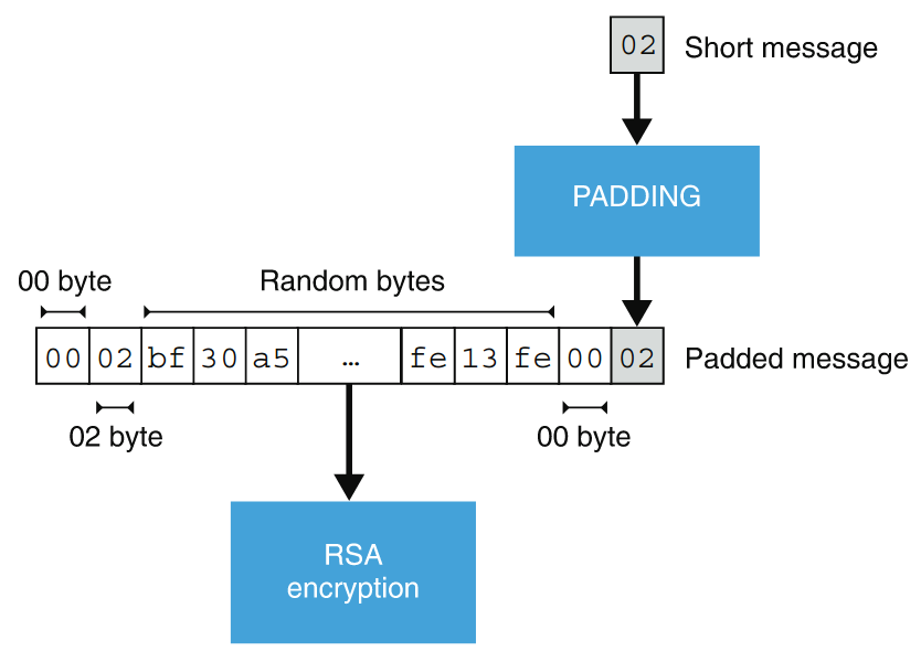
Bleichenbacher made use of the malleability property of RSA in his
million message attack on RSA PKCS#1 v1.5. His attack works by
intercepting an encrypted message, modifying it, and sending it to the
person in charge of decrypting it. By observing if that person can
decrypt it (the padding remained valid), we obtain some information
about the message range. Because the first two bytes are 0x0002, we
know that the decryption is smaller than some value. By doing this
iteratively, we can narrow that range down to the original message
itself.
Even though Bleichenbacher’s attack is well-known, there are still many systems in use today that implement RSA PKCS#1 v1.5 for encryption, and so variants of this vulnerability still exist in many modern servers, now known as the “Return Of Bleichenbacher’s Oracle Threat” (ROBOT) attack.6
References
-
Aumasson, Jean-Philippe. 2017. Serious Cryptography: A Practical Introduction to Modern Encryption. No Starch Press.
-
Boneh, Dan. 1999. "Twenty Years of Attacks on the RSA Cryptosystem." Notices of the American Mathematical Society 46 (2): 203--13.
-
Heninger, Nadia, Zakir Durumeric, Eric Wustrow, and J. Alex Halderman. 2012. "Mining Your Ps and Qs: Detection of Widespread Weak Keys in Network Devices." In Proceedings of the 21st USENIX Security Symposium.
-
Katz, Jonathan, and Yehuda Lindell. 2021. Introduction to Modern Cryptography. 3rd ed. CRC Press.
-
Wong, David. 2021. Real-World Cryptography. Manning Publications.
Please don’t use this for any real-world cryptographic applications!
We won’t cover here how Bleichenbacher’s attack works, but it works similarly to the padding oracle attack against CBC-mode encryption.
You may notice this when you are generating private keys in OpenSSL. It actually encodes \((p, q, d_p, d_q, q^\prime)\) as the private key, not just \((N, d)\).
This is a simpler case of Coppersmith’s attack on low public exponents.
Digital signature schemes
Relevant readings: Katz and Lindell 13.1–13.5, Wong 7.3
Digital signatures
A signature scheme is defined by three PPT algorithms \((\textsf{Gen}, \textsf{Sign}, \textsf{Ver})\):
-
The key-generation algorithm Gen takes as input a security parameter \(\texttt{1}^n\) and outputs a pair of keys \((\textit{pk}, \textit{sk})\). We assume that pk and sk each has length at least \(n\), and that \(n\) can be determined from pk or sk.
-
The signing algorithm Sign takes as input a private key sk and a message \(m\) from some message space (that may depend on pk). It outputs a signature \(\sigma\), and we write this as \(\sigma \getsrandom \Sign{\textit{sk}}{m}\).
-
The deterministic verification algorithm Ver takes as input a public key pk, a message \(m\), and a signature \(\sigma\). It outputs a bit \(b\), with \(b = \texttt{1}\) meaning “valid” and \(b = \texttt{0}\) meaning “invalid.” We write this as \(b \gets \Ver{\textit{pk}}{m, \sigma}\).
Digital signatures vs. MACs
There are two important properties that digital signatures have, which makes them more preferable to MACs in some cases.
First, signatures are publicly verifiable. Recall that since MACs use the same (secret) key to generate a MAC and to verify a MAC, tag verification can only be done by the key holder. Contrast that to signatures, where anyone with the public key can verify a signature.
Second, signatures are non-repudiable. The main idea of non-repudiation is that the signer cannot (easily) deny issuing a signature. In particular contexts, such as for legal applications, non-repudiation is very crucial. MACs cannot provide this functionality!
Digital signatures vs. public-key encryption
It’s tempting to see signatures as the converse of encryption, but they are not. Signing is not the same as encrypting with the private key. Encryption provides confidentiality whereas a digital signature is used to prevent forgeries. The most salient example of this difference is that it’s okay for a signature scheme to leak information on the message signed, because the message is not secret. For example, a scheme that reveals parts of the messages could be a secure signature scheme but not a secure encryption scheme.
Due to the processing overhead required, public-key encryption can only process short messages, which are usually secret keys rather than actual messages. A signature scheme, however, can process messages of arbitrary sizes by using their hash values \(H(m)\) as a proxy (this is the “hash-and-sign” paradigm), and it can be deterministic yet secure.
Security notions for signature schemes
Like MACs, the general security goal of a digital signature is to prevent signature forgery on a new message.
The security notions EUF-CMA (“secure”) and SUF-CMA (“strongly secure”) carry over from MACs, though we need to tweak their definitions a bit.
Fix a signature scheme \(\Pi = (\textsf{Gen}, \textsf{Sign}, \textsf{Ver})\), a security parameter \(n\), and a PPT adversary \(\mathcal{A}\). We define the EUF-CMA game as follows:
-
\(\Gen{\texttt{1}^n}\) is run to generate keys \((\pk, \sk)\).
-
The adversary \(\mathcal{A}\) is given \(\pk\) and oracle access to \(\Sign{\sk}{\cdot}\). The adversary eventually outputs \((m, \sigma)\).
-
\(\mathcal{A}\) wins if and only if \(\Ver{\pk}{m, \sigma} = \texttt{1}\) and \(\mathcal{A}\) never queried \(m\).
A signature scheme \(\Pi\) is existentially unforgeable under a chosen-message attack if \(\Pr[\text{$\mathcal{A}$ wins the EUF-CMA game}]\) is negligible.
RSA-based signatures
RSA can be repurposed as a signature scheme. If you understood how RSA encryption works, then this section should be straightforward because signing with RSA is the opposite of encrypting with RSA:
-
To sign, you encrypt the message with the private key (instead of the public key), which produces a signature (a random element in the group).
-
To verify a signature, you decrypt the signature with the public key (instead of the private key). If it gives you back the original message, then the signature is valid.
Textbook RSA signatures
More precisely, if your private key is the private exponent \(d\), and your public key is the public exponent \(e\) and public modulus \(N\), you can:
-
Sign a message by computing \(\sigma \gets m^d \bmod N\), and
-
Verify a signature by computing \(\sigma^e \bmod N\) and check that it is equal to the message \(m\).
Like with textbook RSA encryption, textbook RSA signatures are also insecure, owing to its malleability. As such, we can do the following sorts of attacks against textbook RSA signatures:
-
Forgery from public key
Choose arbitrary value \(\sigma\), then output \((m, \sigma)\) where \(m \gets \sigma^e \bmod N\).
-
Arbitrary forgery for any \(m\)
Pick \(r\), then compute \(m^\prime \gets r^e m \bmod N\). Query signature for \(m^\prime\): \(\sigma^\prime \gets (r^e m)^d \bmod N = rm^d\). Output \((m, \sigma^\prime r^{-1} \bmod N)\).
Hash-and-sign paradigm
Instead of signing the message itself, we sign the hash of the message. This additional step allows signing of arbitrary-length messages (even beyond what’s supported by the RSA modulus), and protects against signature forgery.
Given a secure signature scheme \(\Pi = (\textsf{Gen}, \textsf{Sign}, \textsf{Ver})\) and a collision-resistant hash function \(H\), we can construct a new signature scheme \(\Pi^\prime = (\textsf{Gen}, \textsf{Sign}^\prime, \textsf{Ver}^\prime)\) as follows:
-
\(\textsf{Sign}^\prime\): \(\sigma \gets \Sign{\sk}{H(m)}\)
-
\(\textsf{Ver}^\prime\): output
1if \(\Ver{\pk}{H(m), \sigma} = \texttt{1}\),0otherwise
The nice thing about this construction is that if our original signature scheme \(\Pi\) is secure and the hash function \(H\) is collision-resistant, then our new signature scheme \(\Pi^\prime\) is also secure.
RSA PKCS #1 v1.5
We have already seen the PKCS #1 v1.5 standard in the context of RSA encryption, but this same document contained a specification for signing with RSA. The signature scheme standardized in that document is pretty much the same as the encryption scheme. To sign, first hash the message with a hash function of your choice, then pad it according to PKCS#1 v1.5’s padding for signatures (which is similar to the padding for encryption in the same standard). Next, encrypt the padded and hashed message with your private exponent. Figure 1 illustrates this process.
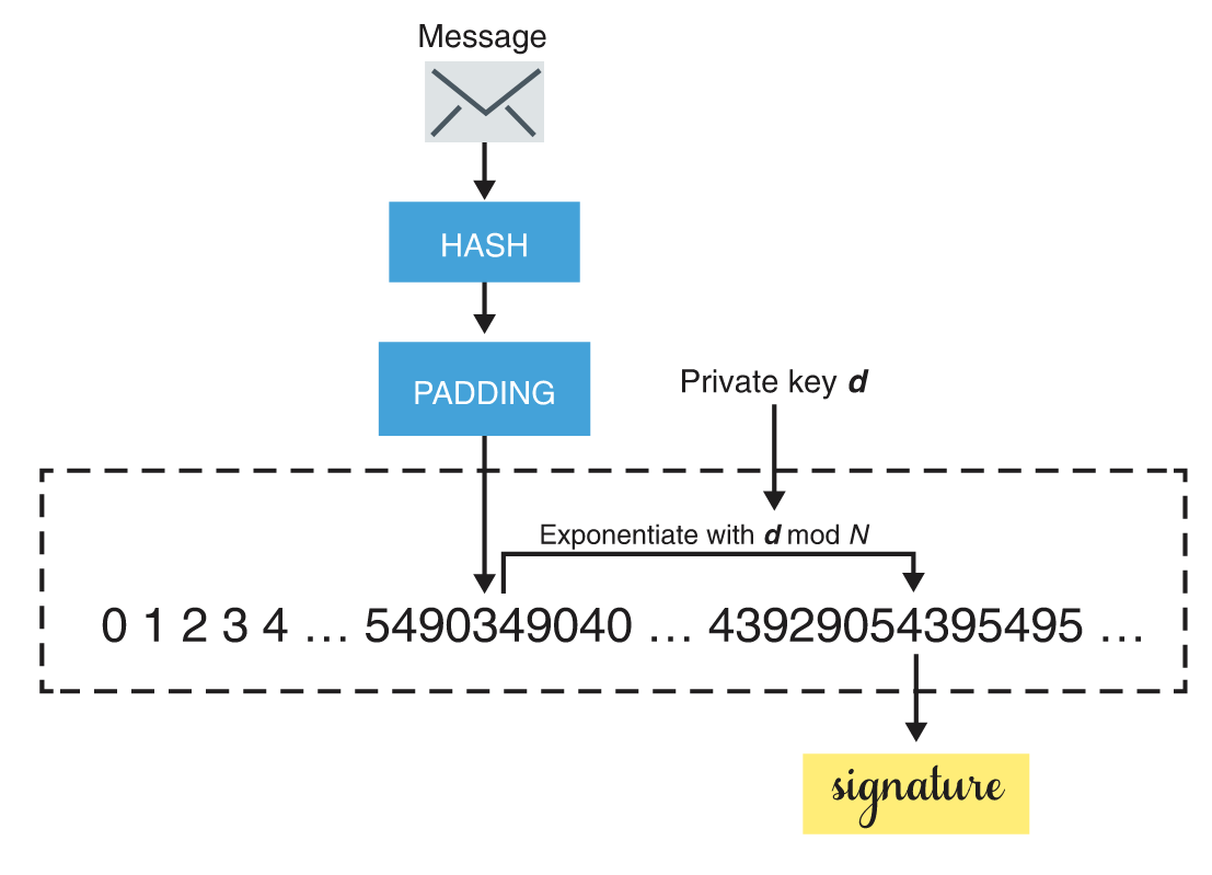
It was mentioned earlier that there were damaging attacks on RSA PKCS#1 v1.5 for encryption; the same is unfortunately true for RSA PKCS#1 v1.5 signatures. In 1998, after Bleichenbacher found a devastating attack on RSA PKCS#1 v1.5 for encryption, he decided to take a look at the signature standard. Bleichenbacher came back in 2006 with a signature forgery attack on RSA PKCS#1 v1.5, one of the most catastrophic types of attack on signatures — attackers can forge signatures without knowledge of the private key! Unlike the first attack that broke the encryption algorithm directly, the second attack was an implementation attack. This meant that if the signature scheme was implemented correctly (according to the specification), the attack did not work.
Unfortunately, RSA PKCS#1 v1.5 for signatures is still widely used. Be aware of these issues if you really have to use this algorithm for backward compatibility reasons. Having said that, this does not mean that RSA for signatures is insecure.
RSA-FDH
The main idea behind Full Domain Hash (FDH) is pretty straightforward: apply a “cryptographic transformation” to messages before signing. This could be done, for example, by applying a cryptographic hash function to the message; as such, it is just a direct application of the hash-and-sign paradigm. To implement it, you simply convert the byte string \(H(m)\) to a number, \(x\), and create the signature \(\sigma \gets x^d \bmod N\). Signature verification is straightforward, too. Given a signature \(\sigma\), you compute \(x' \gets \sigma^e \bmod N\) and compare the result with \(H(m)\).
As the name implies, the hash function used must map onto all possible values of \(\ZZ_N^*\), or in other words, the range of the hash function must be large enough to cover the entire domain of the RSA modulus.
RSA-PSS
The RSA Probabilistic Signature Scheme (PSS) is to RSA signatures what OAEP is to RSA encryption. It was designed to make message signing more secure, thanks to the addition of padding data.
RSA-PSS was standardized in the updated PKCS#1 v2.1 and included a proof of security (unlike the signature scheme standardized in the previous PKCS#1 v1.5). The newer specification (shown in Figure 2) works like this:
-
Encode the message using the PSS encoding algorithm.
-
Sign the encoded message using RSA (as was done in the PKCS#1 v1.5 standard).
Verifying a signature produced by RSA-PSS is just a matter of inverting the encoding once the signature has been raised to the public exponent modulo the public modulus.
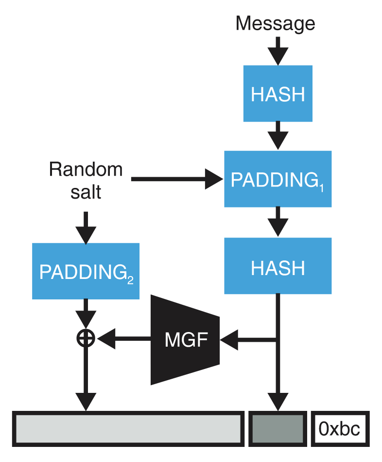
PSS is provably secure, meaning that no one should be able to forge a signature without knowledge of the private key. Instead of proving that if RSA is secure then RSA-PSS is secure, RSA-PSS proves the contrapositive: if someone can break RSA-PSS then that someone can also break RSA. Of course, this only works if RSA is secure, which we assume in the proof.
Compared to FDH, PSS is more complicated, so why bother with the complexity of PSS? The main reason is that PSS was released after FDH, in 1996, and it has a security proof that inspires more confidence than FDH. Specifically, its proof offers slightly higher security guarantees than the proof of FDH, and its use of randomness helped strengthen that proof. These stronger theoretical guarantees are the main reason cryptographers prefer PSS over FDH, but most applications using PSS today could switch to FDH with no meaningful security loss. In some contexts, however, a viable reason to use PSS instead of FDH is that PSS’s randomness protects it from some attacks on its implementation.
Authenticated key exchange
We saw different ways to perform key exchanges between two participants, and we learned that these key exchanges are useful to negotiate a shared secret, which can then be used to secure communications with an authenticated encryption algorithm. Yet, key exchanges didn’t fully solve the problem of setting up a secure connection between two participants as an active man-in-the-middle (MITM) attacker can trivially impersonate both sides of a key exchange. This is where signatures enter the ring.
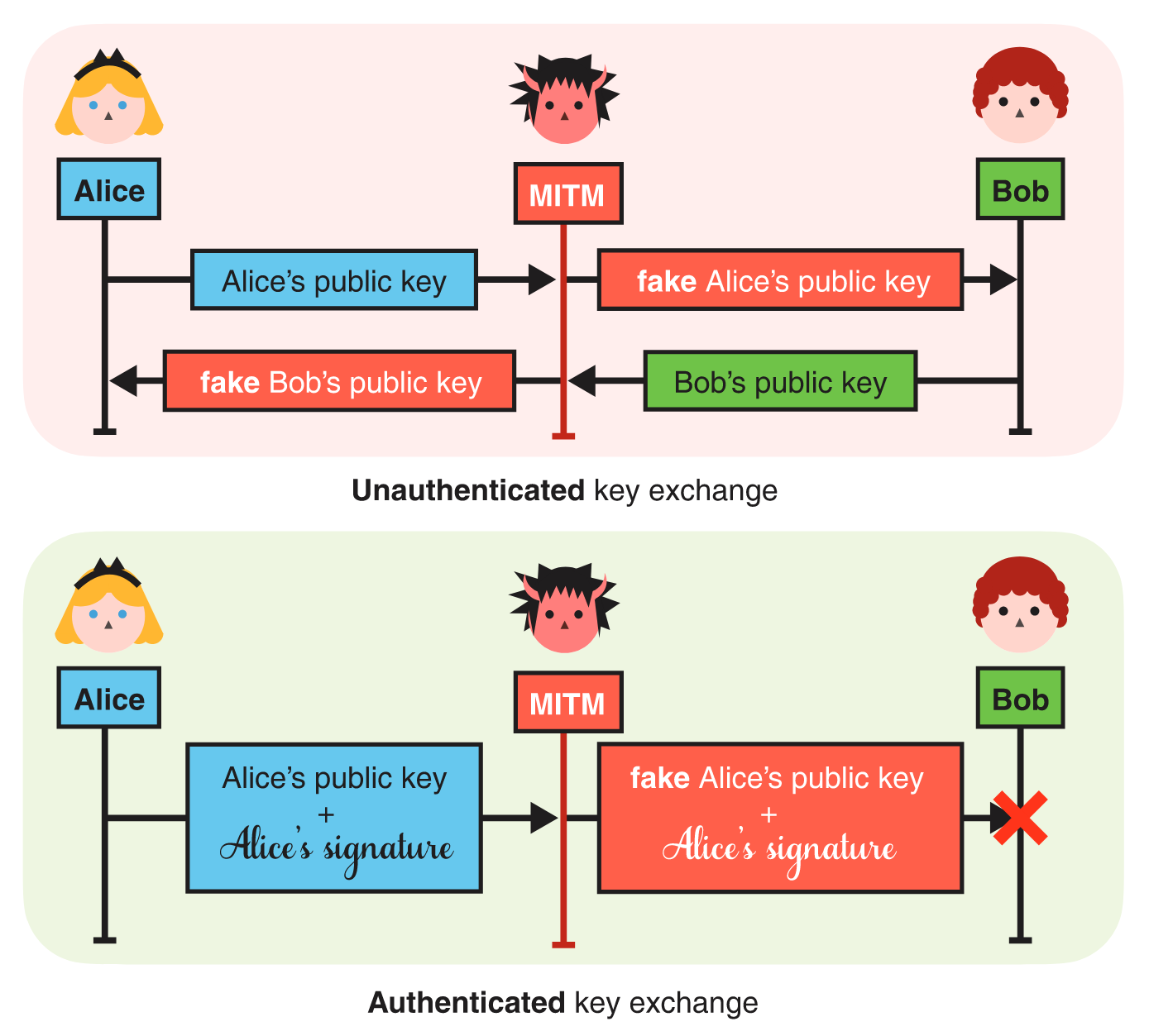
Imagine that Alice and Bob are trying to set up a secure communication channel between themselves and that Bob is aware of Alice’s verifying key. Knowing this, Alice can use her signing key to authenticate her side of the key exchange: she generates a key exchange key pair, signs the public key part with her signing key, then sends the key exchange public key along with the signature. Bob can verify that the signature is valid using the associated verifying key he already knows and then use the key exchange public key to perform a key exchange.
We call such a key exchange an authenticated key exchange. If the signature is invalid, Bob can tell someone is actively MITM’ing the key exchange. Figure 3 shows a comparison between an unauthenticated and an authenticated key exchange.
Note that in this example, the key exchange is only authenticated on one side: while Alice cannot be impersonated, Bob can. If both sides are authenticated (i.e., Bob would sign his part of the key exchange), we call the key exchange a mutually-authenticated key exchange.
References
- Wong, David. 2021. Real-World Cryptography. Manning Publications.
Elliptic curves
Relevant readings: Aumasson ch. 12, Hoffstein, et al. 6.1–6.3, 6.8, Katz and Lindell 9.3.4
Introducing elliptic curve cryptography
Elliptic curve cryptography (ECC) was first introduced in 1985, which paved the way for stronger security with smaller key sizes. It is more powerful and efficient than traditional public-key algorithms like RSA and (classic) Diffie–Hellman, since a 256-bit key in ECC is stronger than a 4096-bit RSA key. It does not deal with the multiplicative group of integers, but rather, it uses a weird mathematical object called an elliptic curve, thus the math behind ECC is a lot more complicated.
ECC did not gain widespread adoption until the early 2000s; the OpenSSL library only added support for ECC in 2005. Most cryptographic applications that rely on the discrete logarithm problem (DLP) will also work when based on its elliptic curve counterpart, ECDLP.
What is an elliptic curve?
An elliptic curve is the set of solutions to an equation of the form $$y^2 = x^3 + Ax + B,$$ where the constants \(A\) and \(B\) must satisfy \(4A^3 + 27B^2 \ne 0\).1 We call the above equation the (short) Weierstrass form, and we occasionally refer to elliptic curves of this form as Weierstrass curves. Figure [fig:elliptic-curves] shows two examples of elliptic curves \(y^2 = x^3 - 3x + 3\) and \(y^2 = x^3 - 6x + 5\).
Despite the name, elliptic curves have absolutely nothing to do with ellipses!
The group law for elliptic curves
One important property of elliptic curves is that the points form an abelian group under point addition.
Point addition
An amazing feature of elliptic curves is that there is a natural way to take two points on an elliptic curve and “add” them to produce a third point, and we can derive the addition law geometrically.
Let \(P = (x_1, y_1)\) and \(Q = (x_2, y_2)\) be points on an elliptic curve \(E\). To get the third point, we draw a line \(L\) that passes through \(P\) and \(Q\). This line \(L\) intersects \(E\) at three points, namely \(P\), \(Q\), and one other point \(R\). We take that point \(R\) and reflect it across the \(x\)-axis (i.e., flip the sign of the \(y\)-coordinate) to get a new point \(R^\prime\). Then \(R^\prime\) corresponds to the sum \(P + Q\). See Figure 1 for a visualization.

To get line \(L\), we recall the point-slope formula from high-school algebra: $$y = \lambda \cdot (x-x_1) + y_1,$$ where the slope \(\lambda\) is equal to \((y_2-y_1)/(x_2-x_1)\). In order to find the points where \(E\) and \(L\) intersect, we substitute \(y\) from the point-slope formula to the original Weierstrass equation and then solve for \(x\).
I’m going to handwave some of the details here, but once you solve for \(x\) from the previous step, we eventually arrive at a formula to get the \(x\)-coordinate of the third point, which we can compute as $$x_3 \gets \lambda^2 - x_1 - x_2,$$ and to get the corresponding \(y\)-coordinate, we just use the point-slope formula as before, but we flip the sign of \(y_1\) to get the reflection along the \(x\)-axis: $$y_3 \gets \lambda \cdot (x_3 - x_1) - y_1.$$
Point negation
If \(P\) and \(Q\) have the same \(x\)-coordinates but not necessarily \(P = Q\), then their \(y\)-coordinates have the same absolute value but with opposite signs. In this case, \(Q\) is the inverse (negation) of \(P\), which we denote as \(-P\).
If we add \(P\) and \(-P\) together, we get the special point called the point at infinity, denoted by \(\mathcal{O}\). Despite the name, the point at infinity actually behaves more like a zero than infinity, thus we consider \(\mathcal{O}\) to be the identity element.
Point doubling
What if \(P = Q\)? Since we have the same two points, they have the same \(x\)-coordinates, which would lead to a division by zero when we try to compute for the slope \(\lambda\). Rather than using the secant line as before, we will instead find the tangent line at point \(P\), as shown in Figure 2.
One way to find the tangent line given some equation is to use implicit differentiation (remember this from your calculus class?); here we implicitly differentiate the Weierstrass equation with respect to \(x\): $$\begin{align} y^2 &= x^3 + Ax + B \\ 2y y^\prime &= 3x^2 + A \\ y^\prime &= \frac{3x^2 + A}{2y}.\end{align}$$ Then \(y^\prime\) would correspond to the slope of the tangent line. To find the specific tangent line passing through point \(P\), we just substitute \(x\) and \(y\) with the \(x\)- and \(y\)-coordinates of \(P\): $$\lambda \gets \frac{3x_1^2 + A}{2y_1}.$$
Once we get \(\lambda\), we can simply apply the previous formulas for \(x_3\) and \(y_3\) to get the “third point.”
Scalar multiplication
Recall that for a multiplicative group \(G\), the exponentiation operation is defined as the result of multiplying an element \(x \in G\) with itself \(k\) times: $$x^k = \underbrace{x \cdot x \cdots x}_{\text{$k$ times}}.$$
If \(k = 0\), then \(x^0 = e\), the identity element of \(G\). For an additive group, exponentiation is called scalar multiplication, as it is defined as the result of adding an element \(x \in G\) with itself \(k\) times: $$kx = \underbrace{x + x + \cdots + x}_{\text{$k$ times}}.$$
Since the points of an elliptic curve form a group under point addition, scalar multiplication for a point \(P\) is then: $$kP = \underbrace{P + P + \cdots + P}_{\text{$k$ times}}.$$ If \(k = 0\), then we get \(kP = \mathcal{O}\), the point at infinity.
In similar fashion to exponentiation by repeated squaring, we can do scalar multiplication efficiently through repeated doubling. We then have a similiar-looking algorithm called the double-and-add algorithm:
DoubleAndAdd(\(P\), \(k\)):
1: if \(k \mathrel{=}0\)
2: return \(\mathcal{O}\)
3: else if \(k\) is even
4: return DoubleAndAdd(\(2P\), \(k/2\))
5: else
6: return \(P\; + \) DoubleAndAdd\((P, k-1)\)
The running time is \(O(\log k)\), or \(O(n)\) where \(k\) is \(n\) bits long.
Just like you can’t really raise a group element to another group element, multiplying two elliptic curve points is undefined.
Elliptic curves over finite fields
So far we have been dealing with elliptic curves over \(\QQ\). If the underlying field is changed to a finite field, we now get a cloud of points instead of a nice, smooth curve. Figure 3 shows the plot of the elliptic curve over \(\FF_{71}\) defined by \(y^2 = x^3 + 13x + 45\).
Despite this change, the group law still holds!
Let \(p \ge 3\) be a prime. An elliptic curve \(E\) over \(\FF_p\) is an equation in short Weierstrass form $$y^2 = x^3 + Ax + B,$$ with \(A, B \in \FF_p\) satisfying \(4A^3 + 27B^2 \ne 0\). The set of points on \(E\) with coordinates in \(\FF_p\) is the set $$E(\FF_p) = \Set{(x,y) \mid x,y \in \FF_p \text{ and } y^2 = x^3 + Ax + B} \cup \Set{\mathcal{O}},$$ where \(\mathcal{O}\) is the point at infinity.
The elements \(E(\FF_p)\) are called the points on the elliptic curve \(E\) defined by the above equation.
Suppose we have an elliptic curve over \(\FF_7\) defined by \(y^2 = x^3 + x + 4\). We first make a list of the possible values of \(x \in \FF_7\), then of \(y^2 \gets x^3 + x + 4\). Note that there is a solution for \(y\) if and only if \(y^2\) is a perfect square in \(\FF_7\), i.e., iff \(y^2\) is a quadratic residue modulo \(7\). $$\begin{array}{c|cc|c} x & y^2 \gets x^3 + x + 4 & y & \text{points} \\ \hline 0 & 4 & \Set{2, 5} & (0,2), (0,5) \\ 1 & 6 & \text{---} & \text{---} \\ 2 & 0 & \Set{0} & (2,0) \\ 3 & 6 & \text{---} & \text{---} \\ 4 & 2 & \Set{3, 4} & (4,3), (4,4) \\ 5 & 1 & \Set{1, 6} & (5,1), (5,6) \\ 6 & 2 & \Set{3, 4} & (6,3), (6,4) \\ \end{array}$$
Therefore, the points in \(E(\FF_7)\) are \((0,2), (0,5), (2,0), (4,3), (4,4), (5,1), (5,6), (6,3), (6,4)\), and the point at infinity \(\mathcal{O}\), having \(10\) points in total.
Elliptic curves over finite fields of prime-power order
If we allow the order of the finite field to be a prime power, i.e., \(q = p^k\) for prime \(p\) and integer \(k > 1\), then the equation takes a different form called the generalized Weierstrass form: $$y^2 + a_1 xy + a_3 y = x^3 + a_2 x^2 + a_4 x + a_6.$$ Note that the short Weierstrass form is a special case, where \(a_1 = a_2 = a_3 = 0\), and \(a_4\) and \(a_6\) correspond to the constants \(A\) and \(B\), respectively.
Computation with elliptic curves in Sage
Suppose \(E\) is an elliptic curve over a finite field \(\FF_q\) in short Weierstrass form: $$y^2 = x^3 + Ax + B,$$ where \(q = p^k\) for prime \(p\) and positive integer \(k\). We can construct \(E\) in Sage using the following syntax:
E = EllipticCurve(GF(q), [A, B])
For example, to define the elliptic curve over \(\FF_7\) defined by \(y^2 = x^3 + x - 1\), we can do:
E = EllipticCurve(GF(7), [1, -1])
E
If the underlying finite field has a prime-power order (i.e., of the form \(p^k\) where \(k > 1\)), then we "expose" another variable, say \(a\), to denote elements in \(\FF_{p^k}\):
FF_27.<a> = GF(3^3)
E2 = EllipticCurve(FF_27, [a^2, a+1])
E2
A point \((x, y)\) is entered using E(x, y), and the point at infinity \(\mathcal{O}\) with E(0).
E(2, 4)  # point (2, 4)
E(0)     # point at infinity
Note that Sage represents points on an elliptic curve using projective coordinates of the form \((X : Y : Z)\), as opposed to affine coordinates of the form \((x, y)\). (More details about using affine or projective coordinates to represent points are discussed here.)
We can do basic arithmetic on elliptic curve points (i.e., addition, negation,
scalar multiplication) using the typical syntax.
P = E(2, 3)
Q = E(4, 2)
R = E(3, 1)
print('-P =', -P)
print('5Q =', 5*Q)
print('P+R =', P+R)
print('R-Q =', R-Q)
To determine the set of points on this curve, we can use the E.points() method.
If you only want the number of points (also called the order of the elliptic curve),
we can use E.order().
print(f'There are {E.order()} points')
E.points()
The elliptic curve discrete logarithm problem
The elliptic curve discrete logarithm problem (ECDLP) is exactly like the “normal” DLP for multiplicative cyclic groups. More concretely, let \(E\) be an elliptic curve over \(\FF_p\) and let \(P\) and \(Q\) be points in \(E(\FF_p)\). Then the ECDLP is the problem of finding an integer \(k\) such that \(Q = kP\).
For some families of curves, the best algorithms known to solve ECDLP are generic group algorithms like Pollard \(\rho\) and baby step–giant step.
Counting points
Counting the number of points on an elliptic curve \(E(\FF_q)\) (also called the order of \(E(\FF_q)\), denoted by \(\Len{E(\FF_q)}\)) efficiently is very tricky. The problem of counting points is of cryptographic relevance, since the hardness of ECDLP depends on the number of points on the underlying elliptic curve. This can help us classify elliptic curves in terms of security levels and thus use the appropriate elliptic curve for the level of security that we actually need.
The absolute maximum number of points of \(E(\FF_q)\) is \(2q+1\) since there could be two points for each \(x \in \FF_q\), plus \(\mathcal{O}\). However, a famous theorem by Hasse establishes a tighter and more useful lower and upper bounds for \(\Len{E(\FF_q)}\):
Let \(E\) be an elliptic curve over \(\FF_q\). Then the order of \(E(\FF_q)\) satisfies $$-2\sqrt{q} \le \Len{E(\FF_q)} - (q+1) \le 2\sqrt{q}.$$
Rearranging this result, we get $$q+1 - 2\sqrt{q} \le \Len{E(\FF_q)} \le q+1 + 2\sqrt{q},$$ which we can then use to get concrete tight bounds.
Elliptic curve Diffie–Hellman (ECDH)
The elliptic curve version of Diffie–Hellman is identical to that of classical Diffie–Hellman but with different notations:
-
Alice and Bob agree upon an elliptic curve \(E(\FF_p)\) of order \(q\) (where \(q\) is \(n\) bits long) and a base point \(P \in E(\FF_p)\).
-
Alice chooses \(a \getsrandom \ZZ_q\) uniformly at random and sends \(h_A \gets aP\) to Bob.
-
Bob receives \(h_A\), then chooses \(b \getsrandom \ZZ_q\) uniformly at random and sends \(h_B \gets bP\) to Alice.
-
Alice receives \(h_B\), and computes the shared key \(k_A \gets a (bP) = (ab) P\).
-
Bob computes the shared key \(k_B \gets b (aP) = (ba) P = (ab) P\).
The security of ECDH follows from the hardness of ECDLP. Diffie–Hellman protocols that rely on DLP can therefore be adapted to work with elliptic curves and rely on ECDLP as a hardness assumption.
Signing with elliptic curves
The standard algorithm used for signing with elliptic curve cryptography is the elliptic curve digital signature algorithm, or ECDSA for short.
As with all such schemes, the public key is pretty much always generated according to the same formula:
-
The private key is a large number \(x\) generated randomly.
-
The public key is computed using \(Q \gets xG\), where \(G\) is a group generator (also called the base point) of order \(n\).
To compute an ECDSA signature, you need a hash of the message you’re signing \(H(m)\), your private key \(x\), and a random number \(k\) that is unique per signature. An ECDSA signature is a pair of integers \((r, s)\), computed as follows:
-
\(r\) is the \(x\)-coordinate of \(kG\)
-
\(s \gets k^{-1} (H(m) + xr) \bmod n\)
To verify an ECDSA signature, a verifier needs to use the same hashed message \(H(m)\), the signer’s public key, and the signature values \(r\) and \(s\). The verifier then:
-
Computes \(u_1 \gets H(m) s^{-1} \bmod n\),
-
Computes \(u_2 \gets r s^{-1} \bmod n\), and
-
Validates that the \(x\)-coordinate of the point \(u_1 G + u_2 Q\) is the same as the value \(r\) of the signature.
The random number \(k\) is sometimes called a nonce because it is a number that must only be used once, and is also sometimes called an ephemeral key because it must remain secret. It is important that \(k\) must never be repeated nor be predictable! Without that, it is trivial to recover the private key.
In general, cryptographic libraries perform the generation of this nonce (the \(k\) value) behind the scenes, but sometimes they don’t and let the caller provide it. This is, of course, a recipe for disaster. For example, in 2010, Sony’s PlayStation 3 was found using ECDSA with repeating nonces (which leaked their private keys).2
ECDSA vs. RSA signatures
RSA’s verification process is often faster than ECDSA’s signature
generation because it uses a small public key \(e\). But ECDSA has two
major advantages over RSA: shorter signatures and signing speed. Using
OpenSSL’s benchmarking tool openssl speed, we can see that signing
with ECDSA is about \(225\) times faster than signing with RSA, mainly
because ECDSA works with much smaller numbers than RSA does for a
similar security level.
brian@thonkpad ~/classes/csci184.03
% openssl speed ecdsap256 rsa4096
Doing 4096 bits private rsa's for 10s: 3228 4096 bits private RSA's in 9.98s
Doing 4096 bits public rsa's for 10s: 180249 4096 bits public RSA's in 9.98s
Doing 256 bits sign ecdsa's for 10s: 417901 256 bits ECDSA signs in 9.95s
Doing 256 bits verify ecdsa's for 10s: 138465 256 bits ECDSA verify in 9.98s
version: 3.0.5
--- snipped for brevity ---
                  sign    verify    sign/s verify/s
rsa 4096 bits 0.003150s 0.000063s    317.4  15900.0
                              sign    verify    sign/s verify/s
 256 bits ecdsa (nistp256)   0.0000s   0.0001s  42627.6  13952.5
The takeaway is this: you should prefer ECDSA to RSA except when signature verification is critical and you don’t care about signing speed, as in a sign-once, verify-many situation (e.g., when digitally signing an app, the developer only needs to sign once, the app’s signature will be verified as many times as the number of devices that would install the app).
Other kinds of elliptic curves
The Weierstrass form is not the only way to define an elliptic curve, and other forms are often used for reasons of efficiency and/or implementation-level security.
Montgomery curves
An elliptic curve in Montgomery form involves equations of the form $$B y^2 = x^3 + Ax^2 + x,$$ where \(B \ne 0\) and \(A \ne \pm 2\). In contrast to the Weierstrass form, not every curve can be expressed in Montgomery form; in particular, the order of any elliptic-curve group written in Montgomery form is a multiple of \(4\).
Twisted Edwards curves
An elliptic curve in twisted Edwards form involves equations of the form $$ax^2 + y^2 = 1 + d x^2 y^2,$$ where \(a, d \ne 0\) and \(a \ne d\). The special case where \(a = 1\) is called the Edwards form. Unlike Weierstrass and Montgomery curves, twisted Edwards curves do not need to define a point at infinity since the point \((0, 1)\) fulfills the role of the identity element.
A nice feature of twisted Edwards curves is that when \(a\) is a square in \(\FF_p\), but \(d\) is not, the addition law is simpler. Given points \(P = (x_1, y_1)\) and \(Q = (x_2, y_2)\), we can compute the sum \(P+Q = (x_3, y_3)\) as: $$(x_3, y_3) = \left( \frac{x_1 y_2 + x_2 y_1}{1 + d x_1 x_2 y_1 y_2}, \frac{y_1 y_2 - a x_1 x_2}{1 - d x_1 x_2 y_1 y_2} \right).$$ No special cases needed!
Other curves
There are lots more curves in use that we don’t have time to discuss, such as Hessian curves, Jacobi curves, and Doche–Icart–Kohel curves. A website called the Explicit-Formulas Database collects all the formulas for doing point addition and scalar multiplication for various forms, almost all of which are heavily optimized for efficient implementation.
Standardized elliptic curves
In practice, we don’t use our own elliptic curves for the same reason we don’t roll our own cryptographic algorithms. To quote the SafeCurves website:3
There are many attacks that break real-world ECC without solving ECDLP. The core problem is that if you implement the standard curves, chances are you’re doing it wrong:
Your implementation produces incorrect results for some rare curve points.
Your implementation leaks secret data when the input isn’t a curve point.
Your implementation leaks secret data through branch timing.
Your implementation leaks secret data through cache timing.
Rather, we typically use one of these standardized curves that have been optimized for efficiency and security.
NIST curves
NIST released a document called FIPS 1864 which introduces the NIST curves under Appendix D “Recommended Elliptic Curves for Federal Government Use.”5 Five NIST curves work modulo a prime number, while ten other NIST curves work with binary polynomials that allow for efficient hardware implementation.
The most common of the NIST curves is the P-256 curve. It is an elliptic curve over \(\FF_p\) for the \(256\)-bit prime \(p = 2^{256} - 2^{224} + 2^{192} + 2^{96} - 1\), defined by the equation \(y^2 = x^3 - 3x + B\) where \(B\) is a specified constant. The prime was chosen to have this form because it allows for efficient implementation of arithmetic modulo \(p\). Letting \(A\) in the defining equation to be \(-3\) allows for optimization of elliptic curve operations. NIST also provides prime curves of \(192\) bits, \(224\) bits, \(384\) bits, and \(521\) bits.
Some people grew suspicious about the constants used for the NIST curves because only the NSA, which created the curves, knows how the constants in their equations were derived, thereby insinuating at the possibility of a backdoor planted by the NSA. However, there is insufficient evidence so far that this is the case.
Curve25519
Introduced by Daniel J. Bernstein in 2006, Curve25519 (pronounced as “curve two-fifty-five nineteen”) is an elliptic curve designed for fast performance and uses shorter key lengths than other curves. Unlike the NIST curves, it has no suspicious constants and can use the same unified formula for point addition and doubling.
More formally, Curve25519 is a Montgomery curve over \(\FF_p\) defined by: $$y^2 = x^3 + 486662x^2 + x,$$ where \(p = 2^{255} - 19\), hence the name. It can also be represented in twisted Edwards form, where it is known as Edwards25519.
Even though Curve25519 isn’t standardized by NIST, it is used everywhere from web browsers such as Google Chrome, to protocol implementations such as OpenSSH.
secp256k1
The secp256k1 curve is defined in SEC 2: “Recommended Elliptic Curve Domain Parameters,”6 written by the Standards for Efficient Cryptography Group (SECG). It gained a lot of traction after Bitcoin decided to use it instead of the more popular NIST curves, due to the lack of trust in the NIST curves.
It is a type of elliptic curve called a Koblitz curve. A Koblitz curve is just an elliptic curve with some constraints in its parameters that allow implementations to optimize some operations on the curve. The elliptic curve is defined by the equation \(y^2 = x^3 + 7\), where \(x\) and \(y\) are defined over \(\FF_p\), and \(p\) is defined as $$p = 2^{256} - 2^{32} - 2^9 - 2^8 - 2^7 - 2^6 - 2^4 - 1.$$ This defines a group of prime order, like the NIST curves.
Practical considerations
Point compression
A shortcoming of using an elliptic curve \(E(\mathbb{F}_p)\) for cryptography is the fact that it takes two coordinates to specify a point in \(E(\mathbb{F}_p)\). However, the second coordinate actually conveys very little additional information.
Instead of spending another \(\lfloor \log_2 p \rfloor + 1\) bits to represent the \(y\)-coordinate, it is enough to simply send a single bit \(\beta\). For short Weierstrass curves, there are two possible solutions to \(y^2 = x^3 + Ax + B\), which are \(b\) and \(p-b\) for some \(b\). We assume here that we have a way to get \(b\) (i.e., find the square roots modulo \(p\)) efficiently, such as using the Tonelli–Shanks algorithm. Notice that either one of \(b\) and \(p-b\) is less than half of \(p\), while the other one is greater than half of \(p\). Based from this observation, we can use the single bit \(\beta\) to indicate which half the \(y\)-coordinate belongs to.
Affine vs. projective coordinates
So far, we represented points on an elliptic curve using affine coordinates, those in the form of \((x, y)\). Another way is to represent points using projective coordinates, as ratios \((X : Y : Z)\).
Points in projective coordinates are instead represented as an ordered triple of numbers \((X : Y : Z)\) where \(X, Y, Z \in \FF_p\). Converting a point (that’s not \(\mathcal{O}\)) between one form to another is easy: $$\begin{align} (x, y) &\mapsto (xz : yz : z), \\ (X : Y : Z) &\mapsto (X/Z, Y/Z).\end{align}$$ The point at infinity \(\mathcal{O}\) can be represented as \((0 : Y : 0)\) for any nonzero \(Y\), for which these are the only points where \(Z = 0\).
The advantage of using projective coordinates is that we can add points without computing inverses modulo \(p\). Suppose we have two points \(P = (X_1 : Y_1: Z_1)\) and \(Q = (X_2 : Y_2 : Z_2)\) where \(P, Q \ne \mathcal{O}\). Then we can express \(P\) and \(Q\) in affine coordinates as $$P = (X_1/Z_1, Y_1/Z_1) \quad\text{and}\quad Q = (X_2/Z_2, Y_2/Z_2),$$ so we can compute \(S \gets P+Q\) (in projective coordinates) as $$S = P+Q = \left(\lambda^2 - X_1/Z_1 - X_2/Z_2 \;:\; \lambda \cdot (X_1/Z_1 - \lambda^2 + X_1/Z_1 + X_2/Z_2) \;:\; 1 \right),$$ where $$\lambda = (Y_2/Z_2 - Y_1/Z_1)(X_2/Z_2 - X_1/Z_1)^{-1} = (Y_2 Z_1 - Y_1 Z_2)(X_2 Z_1 - X_1 Z_2)^{-1}.$$
We’re not necessarily limited to \(Z_3 = 1\) as we did above. In fact, if we let \(Z_3 = Z_1 Z_2 (X_2 Z_1 - X_1 Z_2)^3\) (i.e., multiply each coordinate by this quantity), we can represent \(S\) as $$S = (vw \;:\; u(v^2 X_1 Z_2 - w) - v^3 Y_1 Z_2 \;:\; Z_1 Z_2 v),$$ where $$\begin{align} u &= Y_2 Z_1 - Y_1 Z_2, \\ v &= X_2 Z_1 - X_1 Z_2, \\ w &= u^2 Z_1 Z_2 - v^3 - 2v^2 X_1 Z.\end{align}$$
A potential downside of using projective coordinates is that a point expressed in projective coordinates may reveal information about how that point was computed, which may in turn leak some secret information.
Invalid curve attack
Elliptic curve Diffie–Hellman can be broken if input points are not validated. This is because computing the sum \(P + Q\) given two points does not involve the coefficient \(B\) in any way, as it only relies on the coordinates of \(P\) and \(Q\) and the coefficient \(A\) (when doubling points).7 As a consequence, it is entirely possible to add two points that come from curves with different \(B\) coefficients! This is the main idea behind the invalid curve attack.
To see this attack in action, consider the following scenario involving Alice and Bob using ECDH:
-
Alice and Bob agree upon an elliptic curve and a base point \(P\).
-
Bob sends his public key \(h_B \gets bP\) to Alice.
-
Alice, instead of sending a public key \(h_A \gets aP\) on the agreed upon curve, sends a point on a different curve, either intentionally or accidentally.
Unfortunately, this new curve is weak and allows Alice to choose a point \(Q\) for which solving ECDLP is easy. She chooses a point of low order, for which there is a relatively small \(k\) such that \(kP = \mathcal{O}\).
Alice then sends \(h_A \gets aQ\) instead.
-
Bob receives \(h_A\) and computes the shared key \(k_B \gets b h_A = b(aQ)\).
Bob unknowingly computed the shared key on the weaker curve!
Because \(Q\) was chosen to belong to a small subgroup within the larger group of points, the result \(b h_A\) will also belong to that small subgroup, allowing an attacker to determine the shared secret \(b h_A\) efficiently if they know the order of \(Q\).
An instance of an invalid curve attack is found on certain implementations of the TLS protocol, which uses ECDH to negotiate session keys.
This condition ensures that the equation \(x^3 + Ax + B = 0\) has no repeated roots.
Since the latest draft version FIPS 186-5, Appendix D has been made into a standalone NIST Special Publication 800-16: https://csrc.nist.gov/publications/detail/sp/800-186/draft.
You can even double-check the previous sections to see this is the case.